
Data reporting
No statistical methods were used to predetermine sample size due to the predetermined sample availability of the GTEx project27. Three samples were excluded from the study as they were annotated with the wrong tissue label.
Data acquisition
GTEx WSIs were downloaded from the public portal27. All slides were acquired with a Leica Biosystems Aperio ScanScope with a ×20 objective (effective resolution of ~0.4942 µm per pixel). Demographic data (including the exact chronological age of the individuals), lifestyle information, clinical information for the participants and gene expression data were downloaded from dbGaP because they are under protected access.
Independent histopathological image datasets were used to validate the tissue clocks. Postmortem brains of individuals aged 35 to 99 years were identified from the archives of the Institute of Neuropathology and Neuromolecular Pathology at the Medical University of Innsbruck. Ethical approval for the use of formalin-fixed and paraffin-embedded (FFPE) tissues for research studies, along with a waiver of the requirement for informed consent, was granted by the ethical committee of the Medical University of Innsbruck (EK 1387/2025). FFPE tissues of frontal and cerebellar cortex were retrieved, and hematoxylin and eosin-stained sections were assessed for central nervous system pathology. The sections were then digitized in ×20 magnification using an Aperio GT 450 DX automated digital pathology slide scanner, and whole-slide scans were saved in .svs format. Skin samples were obtained at the Department of Plastic and Reconstructive Surgery or the Department of Dermatology of the Medical University of Vienna. The study complied with national law and was approved by the Medical University of Vienna Ethics Committee (ECS 1969/2021 and ECS 1877/2024), with informed consent obtained from participants. Skin biopsies were fixed in formalin, embedded in paraffin and stored at −20 °C to preserve tissue structure and RNA for morphological and molecular analyses. For histology, FFPE blocks were sectioned into 6-µm slices using a microtome (Leica RM2235) onto SuperFrost Plus slides (VWR, 6310108) and stained with hematoxylin and eosin using a Dako Cover Stainer with standard reagents (Agilent). Slides were digitized in ×40 magnification using a Hamamatsu C9600-12 automated digital pathology slide scanner, and whole-slide scans were saved in .ndpi format. Lung samples were obtained under approval by the ethics committee of UZ Leuven/KU Leuven (S52174), with signed informed consent from participants. The study was conducted in accordance with the Declaration of Helsinki. Whole lungs were excised, air inflated and snap frozen, with all samples derived from the same anatomical region. Slides were scanned on an Axioscan 7 with an EC Plan-Neofluar ×20/0.50-NA M27 objective (effective resolution of ~0.1725 µm per pixel) and saved in .czi format.
WSI processing
WSIs were segmented into foreground tissue and background regions using computer vision algorithms adapted from the preprocessing utilities of the CLAM repository67. Only the image preprocessing components were reused; the CLAM multiple-instance learning and attention-based models were not used. We repurposed and modularized the preprocessing code into a general-purpose WSI library that is model agnostic and now open sourced at https://github.com/rendeirolab/wsi. Briefly, signal from a WSI thumbnail was converted to HED color space, Otsu-thresholded and dilated, and small objects (<500 pixels) were removed. To produce a tissue mask, the holes were filled, and a separate mask for the holes (>0.5 and <50 pixels) was used. Contours were stored in .h5 format, and slides were tiled in the tissue area with square patches of 224 pixels (effective size of ~112 µm).
Vision model fine-tuning
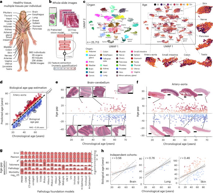
To capture histological features better, we fine-tuned a variety of vision model architectures in a tissue classification task. Importantly, we created a balanced dataset comprising equal numbers of slides and tile patches from different tissues, age brackets and sexes. We built upon well-established and pretrained models (AlexNet, VGG16, ResNet50, ResNet152, ResNet50, ConvNeXt tiny and ConvNeXt base), with a classifier head corresponding to the tissue classes. To train the new classifier head layer, we first froze all layers of the pretrained model and trained one epoch, followed by up to 100 epochs of fine-tuning the whole model via the AdamW optimizer with cosine annealing. We started with an empirically discovered learning rate by measuring the loss at incremental steps and choosing one-tenth of the minimum (learner.lr_find). Model fine-tuning was performed with PyTorch and Fast.ai, either on TPUs through Google Colab or on a workstation with two NVIDIA RTX A6000 GPUs.
Feature extraction and unsupervised analysis
Inference was run on a high-performance computing cluster using CPUs for all tiles in all slides at three levels of magnification (~480 million tiles). We worked with three different tile widths (224, 448 and 896 pixels at ~0.5 µm per pixel) but centered at the same location, such that the tile centroids across different widths were matched and represented different, progressively wider views of the same tissue location. Features were extracted with a variety of models as described earlier, and for downstream analysis, feature values were aggregated across tiles by means and concatenated across different tile widths to generate a single feature vector for each WSI. We used AnnData and Scanpy68 to perform dimensionality reduction with principal component analysis (PCA), compute neighbors and compute a UMAP for visualization, each step with default parameters (PCA: 50 principal components, neighbor graph: 15 neighbors on the basis of PCA representation, UMAP: 0.5 min_dist, 1.0 spread).
Analysis of total variance explained
To provide a global measure of the importance of various factors in explaining the observed range of morphological heterogeneity across tissue samples, we implemented linear models that use those factors to predict the variability of samples in the principal components. We collected 86 variables related to demography, lifestyle, serology, morbidity and circumstances of death for each participant. Regression was based on an ordinary least squares regression model (statsmodels69) and was fit for each tissue and principal component at a time. The full model was fit first, and models missing each of the 86 variables (leave one out) were subsequently fit and compared to the full model on the basis of the adjusted coefficient of determination. These values were weighted by the variance ratio of each principal component in the data and summed across components to generate a value of total variance explained for the factor.
Tissue clocks and estimation of age gaps
We used linear models implemented in scikit-learn70, including Linear Regression, Ridge, RidgeCV and RandomForestRegressor, using GroupKFold (k = 5) cross-validation, where the group was an individual, to ensure that the training and validation splits did not contain the same individual. Models were trained for each tissue separately using the features from the vision models as inputs, age as the target and sex, cohort type and minutes of ischemic time as covariates. To assess potential overfitting, we also fitted the models on shuffled age labels as target. We computed the coefficient of determination and MAE as metrics. Adjustment for regression to the mean was performed by regressing out the coefficient of age from the observed residuals as previously described16. All the results reported downstream were obtained for tissue clocks trained with a Ridge model, as it exhibited good performance and was fast.
The ‘Bladder’, ‘Cervix – Ectocervix’, ‘Cervix – Endocervix’, ‘Fallopian Tube’ and ‘Kidney – Medulla’ tissues had fewer than 100 samples available and overall showed poor performance (for example, MAE > 9 years) and were excluded from further analysis. We also noticed that three samples had extreme age-gap values (‘GTEX-1GMR2-0426’, ‘GTEX-1S82U-0426’ and ‘GTEX-11ZTS-0426’), which, upon inspection, were found to be annotated with the wrong tissue type.
Classic vision and foundation models
To validate and assess the generalization of findings with our fine-tuned model, we used 6 classic vision models trained on ImageNet (Supplementary Fig. 5) and 18 pathology foundation models (Extended Data Fig. 3)21,22,35,36,71,72,73,74,75,76,77,78,79,80,81,82,83,84,85,86,87,88,89,90,91,92,93,94. We performed feature extraction using LazySlide95 on NVIDIA H100 GPUs, using square patches of 224 pixels and aggregating features within each slide by the mean (as done previously for our fine-tuned model). Age predictors were fitted as described in the section above using the Ridge model with GroupKFold (k = 5) cross-validation, and metrics were calculated based on the chronological age of the individuals.
GNNs
To further validate the choice of feature aggregation across patches of the same slide, and to enable the visualization of weights associated with biological age on tissue images, we also used GNNs for biological age prediction from histopathological images (Supplementary Fig. 7). Here, tissue patches were used as nodes with features from the convNeXt fine-tuned model. A k-d tree was used for quick nearest-neighbor lookup with a radius of patch size × the square root of 2 to connect adjacent tissue tiles.
The model architecture was composed of a dropout layer (with a probability of 0.1, 0.25 or 0.5), a variable number (2, 4 or 8) of graph convolutional layers (torch_geometric.nn.conv.GCNConv) with batch normalization and ReLU activation. The convolutional layers had a variable number of hidden dimensions (32, 64, 128 or 256) and were aggregated via jumping knowledge (torch_geometric.nn.models.JumpingKnowledge) across all layers, upon which an attention aggregation layer (torch_geometric.nn.aggr.AttentionalAggregation) with sigmoid activation was added. Finally, a fully connected linear layer was added to output a scalar value.
The target value was chronological age, and GNNs were trained per organ for 80 epochs on an NVIDIA A6000 using an 80–20 dataset split, MAE loss, the AdamW optimizer with cosine annealing, with a starting learning rate of 1 × 10⁻³, and weight decay of 1 × 10⁻⁴. We assessed performance in the validation set using MAE, Pearson correlation and coefficient of determination in relation to the known chronological age of the donors.
To visualize attention weights on tissue (Supplementary Fig. 9d), we extracted node-level attention scores from the best-trained GNNs for each tissue. For each patch (node), we obtained the raw gate outputs and normalized them into per-node attention weights using scatter-based softmax over the batch dimension. The outputs were aligned back to the spatial positions of the original patches, and the normalized attention weights were overlaid on the corresponding histological tissue images as heat maps. This enabled spatial visualization of regions that contributed most strongly to the graph-level age prediction.
Telomere lengths and annotated levels of tissue pathology
We leveraged the telomere quantity index values measured for tissue blocks from the same tissues and individuals in the GTEx cohort34. We z scored these values per tissue to account for intertissue variability in the mean values. Only tissues with at least 100 paired WSIs and telomere length samples were used for analysis.
We also leveraged the pathological notes available in the GTEx cohort, in particular the discretized set of 57 text categories describing the WSIs, which comprised 11,016 instances of a term annotating an image. For the purpose of associating particular pathological annotations with histological age gaps, we excluded ‘clean_specimens’, ‘no_abnormalities’ and ‘tma’. For pathologies common across more than one tissue, we also derived an overall ‘body pathology burden’, which is a composite measure of the number of pathologies annotated in all tissues of an individual.
Text term characterization of age gaps
We used the pathology language and image pretraining (PLIP) model35 to embed 512-pixel-wide (at ~0.5 µm per pixel) tiles from every slide in the GTEx project and used them to query the similarity to a set of histological and pathological terms. The terms were selected to represent equal parts of the histological components and features of the various tissues under study (for example, epithelium, muscle, neurons, adipose tissue and myofiber degeneration). The values were aggregated by means per slide, and associations with histological age gaps were derived via regularized linear regression (Ridge).
To assess the agreement between vision-language models in their interpretation of histopathological images of aging, we compared the outputs of PLIP and CONCH using slides from the colon, lung and skin tissues in the GTEx dataset (n = 4,368). For each slide, we computed the cosine similarity of image features to a curated set of 150 histological and pathological text terms using both models. The resulting slide-level similarity matrices were used to compute, for each text term, the Pearson correlation coefficient between the PLIP- and CONCH-derived similarity values, yielding a distribution of model agreement across terms. To identify factors underlying this agreement, we extracted a set of text-level features describing the linguistic structure of each term, including character and word composition (for example, number of characters, word length, punctuation, uppercase and lowercase usage, lexical diversity and character entropy). In addition, we included the mean and standard deviation of the PLIP and CONCH similarity values for each term. These features were standardized and used as predictors in a linear regression model explaining the correlation between models. Finally, we quantified, for each tissue, the association of change in text-term similarity with donor age and the agreement of terms between the vision-language models.
DNA methylation clocks
We used the PyAging package96 to predict the biological age of the DNA methylation samples matched to the histological images of the tissue. DNA methylation data42 were measured via the Infinium HumanMethylationEPIC bead chip, which measures approximately 850,000 CpG sites. We then derived age gaps by comparing them to the real chronological age of the samples and compared both the predicted values and the DNA methylation-derived age-gap values to the histological predictions using Pearson correlation coefficient.
Gene expression analysis
We used bulk gene expression data from the GTEx project that were matched to the same tissues as the histopathology images. We converted gene-level counts to log counts per million (log (CPM)), and any technical replicates were aggregated by means. To explain both aging and tissue-specific rates of age acceleration (age gaps) with gene expression of the corresponding tissues, we implemented Ridge regression using, as previously described, sex, cohort and minutes of ischemic time as covariates. Genes with an absolute coefficient value above 0.005 (> 5% change per decade) were selected. Finally, we used Enrichr97 through the GSEApy package98 for gene set enrichment with the MSigDB database separately for the up- and downregulated gene sets.
Similarly, we also used the 50 MSigDB pathways together with a set of 50 age-related signatures previously compiled (available at https://github.com/WJPina/HUSI/), as well as a set of genes related to extracellular matrix biology, and quantified them in the transcriptomes using the Scanpy function sc.tl.score_genes. This allowed us to obtain a reduced set of broadly and specifically relevant transcriptional features for each sample. We then calculated their association with chronological age or histologically derived biological age per organ and compared the coefficients between the two per organ, as well as the mean across organs, and assessed whether their signed deviation differed using a Wilcoxon test.
Association of tissue-specific age gaps with individual factors
To visualize individuals in groups with differential patterns of biological aging across the various tissues profiled per individual (Fig. 4b), we selected the tissues with abnormally large age gaps (standard deviation of ≥3), set the remaining tissues to 0 and performed PCA, computed neighbors and performed a UMAP as described previously.
To statistically associate individual age gaps with individual-specific factors, we fitted regularized linear models (Ridge) per tissue and sex with factors explaining tissue-specific age gaps. To avoid collinearity, we excluded the following variables: ‘Abnormal WBC’, ‘Drugs For Non Medical Use In 5 y’, ‘HBcAb IgM’, ‘HIV 1 NAT’, ‘HIV I II Ab’, ‘HIV I II Plus O Antibody’, ‘Nephritis, Nephrotic Syndrome and/or Nephrosis’, ‘Night Sweats’, ‘Open Wounds’, ‘Received Human Growth Hormone’ and ‘Tattoos Done In 12 m’. Furthermore, we retained only factors with more than three individuals per tissue and sex.
Tissue clock application to external cohorts
To validate and assess the generalization of the tissue clocks, we investigated additional cohorts for which histopathological images were collected (from brain, lung or skin tissue). In these cohorts, WSI processing was performed in the same manner as in the GTEx cohort, but we ran both our own fine-tuned model as well as foundational models for feature extraction and aggregated the features across patches of each image by the mean. To identify whether the effect of aging could be detected in each cohort, we performed PCA, as well as fitted regression models using the PCA space as a predictor of age to assess the variance explained by donor age.
We then applied the trained tissue clocks from GTEx to the new cohorts, without adding covariates or adjustment for regression to the mean. We performed this not only for models matched by tissue/organ (that is, applying the model trained on GTEx skin samples to the skin cohort) but also across tissue/organ (that is, applying the model trained on GTEx skin samples to the brain cohort).
For the cohort of lung tissue donors, we also used DNA methylation data, which were collected from the same tissue blocks as the histopathological images. Three well-established DNA methylation clocks were used (Horvath, Hannum and PhenoAge) to generate biological age and age-gap predictions. These DNA methylation predictions were contrasted with the predictions from histological images to quantify the agreement between assays and biological age predictors.
To investigate how different regression approaches generalize in the task of cross-cohort prediction, we systematically evaluated a diverse set of regression models spanning linear, nonlinear and ensemble approaches. Linear models included Ridge (L2 regularization), Lasso (L1 regularization) and Elastic Net (combined L1/L2 penalties via ElasticNetCV), as well as Bayesian Ridge regression for automatic regularization tuning. To account for potential outliers among donors, we tested robust regression approaches (Huber and Quantile regressors). Generalized linear models (Gamma and Tweedie regressors) were included to explicitly model the positive, potentially skewed distribution of age. We further evaluated support vector regression (SVR and LinearSVR), random forest and gradient-boosted trees (LightGBM). Finally, we tested multilayer perceptron neural networks in three configurations: standard, with L2 regularization and early stopping and with a custom L1 regularization to promote sparse weight matrices, also with early stopping. All models were compared on their ability to generalize age predictions to independent held-out cohorts via MAE to chronological age.
Agreement and calibration assessment
To quantify the performance of the GTEx-trained tissue clocks on external cohorts, we used Bland–Altman analysis to assess agreement between predicted biological age and chronological age. For each tissue-specific clock applied to each external cohort, we computed (1) the bias, defined as the mean difference between predicted and chronological age, with 95% confidence interval; (2) the limits of agreement, computed as bias ± 1.96 × the standard deviation of differences; and (3) the standard deviation of differences. Additionally, we assessed calibration by fitting a linear regression of predicted age on chronological age for each cohort and tissue, extracting the slope (ideally = 1.0) and intercept (ideally = 0), both with 95% confidence intervals, along with the coefficient of determination (R2). Results were visualized using Bland–Altman plots showing the mean of predicted and chronological ages (x axis) versus their difference (y axis), with reference lines for bias and limits of agreement.
Prediction of age gaps from blood gene expression
We used bulk gene expression data from the GTEx project that were matched to the same tissues as the histopathology images. Blood gene expression profiles were log transformed and converted to CPM (log (CPM)). We filtered genes with low expression by removing those with a mean log(CPM) of <1 (leaving 11,859 genes) and aggregated the technical replicates by means. Because we observed an effect of the aging process on gene expression in general, we opted to first regress out the effect of age from the blood gene expression profiles using regression. We then fitted regularized regression models to predict tissue-specific age gaps from blood gene expression using Ridge models with two cross-validation loops (RidgeCV): one external Kfold (k = 5) that separates different groups of individuals and where standard scaling is applied and one internal Kfold (k = 5) for α-hyperparameter optimization (chosen from 10−1 to 107 in 20 uniform steps). This process was performed independently for each tissue, and for the mean age gap across the tissues of an individual (systemic clock).
For validation, we obtained a comprehensive set of bulk gene expression profiles from samples of peripheral blood mononuclear cells, leveraging the ARCHS4 database52, version 2.2. Gene expression counts were log transformed, normalized in relation to the total, standardized and scaled for each gene, and the coefficients derived for each predictor in the GTEx cohort were applied in a linear model to make age gap predictions for the bulk RNA-seq samples. The primary metric selected to evaluate performance between each disease and healthy samples was a two-tailed t-test with Benjamini–Hochberg false discovery rate correction. This was used due to the fact that our regression models output continuous values (age gap), which are Gaussian and centered at 0, as those were learned from the residuals of our tissue-clock models. We also evaluated the utility of the blood-based predictors in a binary setting by thresholding the age gaps at 1 and calculating the area under the receiver operator curve and the positive predictive value/precision for separating healthy individuals from those with a disease.
Reporting summary
Further information on research design is available in the Nature Portfolio Reporting Summary linked to this article.