End-to-end multimodal pathology foundation model with clinical dialogue

Training data

Institutional review board approval was not required for the research described in this study. This study was conducted retrospectively from deidentified data licensed to Paige.AI Inc. from MSK. The data used in this study were all collected originally for clinical use by MSK in the practice setting and are, therefore, considered secondary data. Only data previously deidentified by MSK were utilized in the analysis, and unique patient identifiers were completely removed from the analytical dataset. To our knowledge, MSK has not transferred any data for which the applicable patient has not consented to or otherwise agreed to MSK’s Notice of Privacy Practices or a substantially similar notice, waiver or consent.

The training data comprise 685,507 specimens collected from 200,692 patients. Each specimen is associated with a report and one or more WSIs, totaling 685,507 reports and 2,350,518 slides. The WSIs were formalin-fixed and paraffin-embedded, stained with routine H&E and scanned at ×20, 0.5 microns-per-pixel, using Leica scanners. The data represent a diverse collection of tissues and diagnoses (Fig. 2). Specimens are from MSK (internal) as well as external institutions (submitted, spanning multiple continents); all specimens are scanned, but not stained, and reported at MSK. Each modality is preprocessed to prepare for model training.

Whole-slide tissue segmentation is performed with a trained fully convolutional network developed on pathologist-annotated slides for use with Paige products, with postprocessing via Otsu thresholding with thresholds of (0.4, 0.5). WSIs are processed at ×20 magnification with a size of 224 × 224 pixels, discarding any tiles that are less than 65% tissue. The resulting tiles are then processed by Virchow2 (ref. ¹) to produce ‘tile embeddings’, the 1,280-dimensional class token output of the model. The distribution of tiles per specimen is very long tailed, as some parts have a large number of WSIs. To prevent training batches from comprising only a few samples, while aiming to not remove specimens, during training, up to 100,000 tile embeddings are loaded per specimen. In cases where specimens have more than 100,000 tile embeddings (approximately 12% of samples in the training dataset), tile embeddings corresponding to WSIs in the specimen are loaded in a random order until the point at which loading all of the tile embeddings for the next WSI would exceed the budget of 100,000. This ensures that partial WSIs are not used. During inference, when batch diversity is no longer a concern, all tiles are loaded. Preprocessing for downstream tasks matches the training preprocessing except for gastrointestinal tasks, where the tissue inclusion criterion is dropped to 10% to enable better coverage of tissue boundaries, which may be important for detecting Helicobacter pylori. Raw report data are delivered at the case level. Regular expression (regex) matching is performed to match the report text, which is labeled with part numbers, to the proper set of WSIs, also labeled with part numbers, for that specimen. The reports are a mix of synoptic worksheets and free-text and are stripped of boilerplate content such as headers/footers, disclaimers and repetitious formatting characters.

Creating clinical dialogue for training

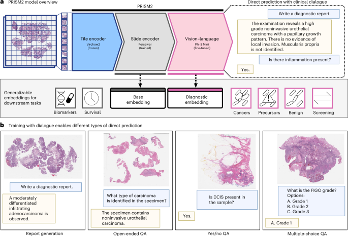
To create high-quality text data for training, we apply GPT-4o⁴³ with various prompting strategies to the report data (see Fig. 2 for an example workflow). We create five classes of processed text tasks to be used in training:

1. (1)

   Clinical report generation. Given a task string (that is, ‘Write a report’), the model must generate the clinical report.

2. (2)

   Yes/no question answering. Given a binary user question, the model must generate an answer.

3. (3)

   Open-ended question answering. Given an open-ended user question, the model must provide an answer.

4. (4)

   Multiple-choice question answering. Given a user question and a list of answer options, the model must select the correct option.

5. (5)

   Image−text matching. Given a report, the model must identify if the report accurately describes the given WSIs and then generate the correct report if they are mismatched.

We choose these templates to broaden the training distribution beyond the obvious report generation task and enable dialogue-based interactions with the trained model. The process to create the data for each of these tasks is described below, and the full system prompts can be found in Supplementary Note 5.

Clinical report rewrites

Using the synoptic reports and free-text notes, we prompt GPT-4o to rewrite all input text, including patient history and specimen description when available, into natural language sentences while retaining all diagnostically relevant findings.

Yes/no question−answer pairs

Question−answer pairs are generated through a multistep process. First, GPT-4o is prompted to convert clinical reports into lists of individual findings, similar to MAIRA-2 (ref. ⁴⁴), which are then filtered to exclude molecular and IHC results. These filtered findings are then used as input to GPT-4o with a prompt to generate question−answer pairs for each finding that can be answered with simply ‘Yes’ or ‘No’. Although effective, we found that this process is naturally biased toward creating questions that have the answer ‘Yes’. We expect that this is because negative findings are typically not mentioned in the reports. For instance, a report positively identifying DCIS in breast tissue allows GPT-4o to generate a pair such as: ‘Q: Is DCIS present? A: Yes’. However, a normal breast tissue report does not mention DCIS, so no negative question−answer pair of the form ‘Q: Is DCIS present? A: No’ is generated, biasing the dataset (and resulting model) toward affirmative responses. Inspired by Goyal et al.⁴⁵, to mitigate this bias we implemented a simple method to mine complementary images for additional questions. Specifically, we pair random reports with random questions and prompt GPT-4o to answer based on the provided report. This yields complementary image−question−answer triplets, balancing the data distribution.

Open-ended question−answer pairs

Open-ended question−answer pairs are also generated from the list of findings described above. We instruct GPT-4o to create the question−answer pairs such that the questions are not answerable with just yes/no but require more specific answers. Open-ended question−answer pairs help mimic more realistic model interactions and improve the diversity of the training data.

Multiple-choice question−option−answer triplets

Multiple-choice question−option−answer triplets are generated from the synoptic reports and free-text notes. We prompt GPT-4.1 (ref. ⁴⁶) to first classify a given report into one of 90 possible CAP Cancer Protocol Templates and then to create as many question−option−answer triplets as possible from the report such that they follow the inferred protocol. We only provide the name of the 90 possible protocols and not the full template as we rely on the inherent recall of these protocols by GPT-4.1.

Image−text matching

The matching task uses the clinical report rewrites described above and does not require further preprocessing. This task aims to force the data to use the image information to complete the task.

PRISM2 architecture

The overall architecture of PRISM2 consists of a slide encoder, a language encoder and a language model, as illustrated in Extended Data Fig. 1 and described below.

Slide encoder

The slide encoder uses a perceiver²¹ architecture. The PRISM2 perceiver uses one block, defined as a cross-attention layer between latent queries and tile embeddings followed by six self-attention transformer layers for the latent queries. acGQA⁴⁷ is used in the tile embedding cross-attention. The number of latent queries is set to 256, and an attention pooling layer is used on these to produce the embedding used in the contrastive objective. This embedding is referred to as the ‘base’ embedding. The perceiver and attention pooler have 541 million and 79 million parameters, respectively.

Language encoder

BioGPT²² is used as the language encoder. We initialize a learnable class token that is concatenated with the input text sequence. The final layer hidden state of the class token is used as the text embedding for the contrastive objective after a linear projection and L2 normalization.

LLM decoder

For the dialogue-focused language model component, we use Phi-3 Mini²⁰, a 3.8-bilion-parameter decoder-only LLM. We adopt a LLaVa-style⁴⁸ approach to enabling Phi-3 Mini to process both images and text. The 256 latents outputted by the slide encoder are further processed by a two-layer multilayer perceptron (MLP) adapter (29 million parameters) to project them into the Phi-3 embedding space and are inserted into the text token embedding sequence as input to the LLM. This allows Phi-3 to integrate the slide and text information via its self-attention layers. In addition to decoding the language tokens, we also perform analysis with the Phi-3 Mini final layer hidden state of the <∣assistant∣> token. We refer to this as the ‘diagnostic’ embedding.

PRISM2 training

Objectives

PRISM2 is trained with both contrastive and autoregressive objectives. Following refs. ^15,23, the contrastive loss is

where N is batch size, τ > 0 is a learned temperature and (v_i, t_i) are the image and text representations, respectively, as defined above. Only the diagnostic report rewrites are used as the text input for the contrastive objective. For the autoregressive objective, we apply the standard cross-entropy loss on next-token predictions from Phi-3 Mini. We use the chat templates as the text input and apply the loss only to the assistant regions of the templates:

where \({\mathcal{A}}\) is the set of token indices corresponding to assistant tokens and X are the image latents after the LLM adapter MLP. The losses are linearly combined to create the total loss:

Data sampling

For the contrastive objective, report rewrites are randomly sampled from five rewrites per report. For the autoregressive objective, we adopt the Phi-3 (ref. ²⁰) chat template using alternating user and assistant tags. The first user message always contains the WSI latents from the slide encoder followed by an initial prompt. In each template, the patient history and specimen description are randomly included, each with a probability of 20%, to allow for conditioning the model on this extra context without being overly reliant on it. Complementary question−answer pairs are included with a sampling rate of 20%. In total, we create 685,000 report rewrites for as many specimens and 14 million question−answer pairs.

Optimization

We adopt a two-stage training approach. In the first stage, the slide encoder, attention pooler, LLM adapter and BioGPT weights are updated using the full objective. The Phi-3 Mini weights are constant (frozen) during this stage. We set λ_con to 0.25 and λ_chat to 1.0. In the second stage, the contrastive objective is discarded, and the slide encoder weights are frozen. The LLM adapter and Phi-3 Mini are updated to allow the language model to better integrate the perceiver latents and model the language of pathology. The optimizer and learning rate schedules are reset for this stage.

We train the model on 56 A100 40GB GPUs with bf16 precision. We use the AdamW⁴⁹ optimizer with β₁ = 0.9 and β₂ = 0.95 and a learning rate warmup for 500 steps, which is then held constant. We do one epoch of stage 1 training with a post-warmup learning rate of 1.0 × 10⁻⁴ on all trainable components except the language encoder, which uses a learning rate of 2.0 × 10⁻⁵ and a 0.1 decay on the slide encoder weights. The large language encoder (Phi-3 Mini) weights are kept frozen in stage 1, but all dialogue objectives are applied. We do 16 epochs of stage 2 training with 500 steps of learning rate warmup to 2.0 × 10⁻⁵ and no weight decay. The slide and language encoders (perceiver and BioGPT) are frozen, and the large language encoder (Phi-3 Mini) is unfrozen for fine-tuning. An epoch is defined as one pass over each of the four chat templates per specimen, for all specimens in the training data. Because the contrastive objective aligns the image representation with the report and not with each chat template, each specimen is paired with its report four times in a single epoch. Several engineering changes were required for efficient training (see Supplementary Note 6 for details).

Survival fine-tuning

The PRISM2 slide encoder was fine-tuned on a large dataset of 225,597 cases with overall survival event data, containing 69,114 death events. Survival prediction is trained by learning a new cross-attention pooling in the (perceiver) slide encoder for ‘survival’ embeddings instead of ‘base’ embeddings and adding a linear regression head on top. This head predicts the log-relative hazard, along with the event time in months, for the partial log-likelihood loss, completing the Cox proportional hazards model. We used the AdamW⁴⁹ optimizer with β₁ = 0.9 and β₂ = 0.98 and a learning rate warmup for 4,000 steps, which is then held constant. We used a post-warmup learning rate of 1.0 × 10⁻⁴ for the slide encoder and 1.0 × 10⁻³ for the prediction head, with a 0.0001 weight decay. The comparison survival specialist model was trained from scratch using the same architecture with the same hyperparameters as stage 1 PRISM2 training.

Comparison models

Several slide-level or part-level embedding models were previously reported and are used for comparison. We describe each in brief here. PRISM¹⁵ is the previous model developed by the PRISM2 team. It differs from PRISM2 in that it is trained using few samples, with fewer types of text outputs and a different training algorithm. TITAN¹⁶ is a slide-level embedding model that uses vision−language pretraining. TITAN aggregates CONCH⁵⁰ in a three-stage processing using both synthetic captions and medical reports and a training dataset of approximately 340,000 WSIs. COBRA³⁶ uses tile representations from four different foundation models to serve as feature space augmentations for a contrastive self-supervised learning approach. COBRA aggregates tiles using a state space architecture and is trained using approximately 3,000 slides. Prov-GigaPath³⁷ uses a vision-only approach to creating a slide-level model. Tile embeddings are aggregated using a masked autoencoding approach and a training dataset of approximately 170,000 WSIs. Virchow2 mMean refers to a baseline where the Virchow2 (ref. ¹) tile embeddings are naively aggregated by simply averaging them all together. Both PRISM2 and COBRA aggregate Virchow2 tile embeddings.

Evaluation methods

Prompt-based inference with question answering

Prompt-based inference with question answering refers to a setting without additional training and includes multiple-choice and yes/no settings. With both yes/no and multiple-choice question answering, we can quantify the probability of predictions. For each classification task, we choose a question prompt w_<i (for example, ‘Is malignant tumor present?’) and consider a set C of possible completions c. For yes/no question answering, these are ‘Yes’ or ‘No’; for multiple-choice question answering, these are the letter options (for example, ‘A’ and ‘B’). The prompts and corresponding tasks are reported in Supplementary Tables 3 and 4.

Formally, we define our dialogue-based prompt-based inference with generative likelihood scoring as

where c is a completion in a set of completions C that cover all classes in the task; w_<i is a tokenized prompt containing a question; and x is the context that contains WSI embedding tokens from the slide encoder.

Contrastive classification

We evaluate prompt-based inference with PRISM and TITAN using the methodologies reported by the authors, respectively. Generally, both models take the approach of considering the cosine similarity score between the slide embedding v and a set of class-specific prompts \({\{{{\bf{t}}}_{c}\}}_{c = 1}^{C}\) and selecting the class that corresponds to the highest similarity:

The softmax function is used to transform cosine similarities to probabilities, enabling the calculation of AUC. For additional details on the contrastive methodology, see the original publications. The prompts for each task, which are specific to the model, are reported in Supplementary Tables 5 and 6.

Linear probe

Beyond prompt-based inference, model embeddings are also evaluated by training a linear classifier or linear regression. To do so, model embeddings are generated, without any text prompting, for training, validation and testing sets of data. Linear classifiers are trained to convergence for each of 24 L2 regularization weights, and the best classifier is selected using the validation set. For survival analysis, a Cox proportional hazards model is fitted to the training set for each of 24 elastic regularization weights (L1 and L2, with an L1:L2 ratio of 0.0001), with the best regressor selected on the validation set.

Report completion

We demonstrate the completion of pathology reports with the CAP worksheet for biopsies with invasive carcinoma of the breast⁴⁰. The specimen procedure and laterality fields and the tumor position field are omitted from this analysis, as they constitute sample collection information rather than diagnostic findings derived from H&E-stained slides. The mitotic rate measurement is also excluded as the model was not trained to count. Filling the fields in the CAP template is posed as prompt-based inference, as described earlier in this section, with multiple-choice question answering for multiclass fields (for example, histologic type and histologic grade) and with yes/no question answering for binary and multilabel fields (for example, presence of DCIS or its architectural pattern). The prompts and corresponding tasks are reported in Supplementary Tables 3 and 4. In total, the report can be represented with nine sets of fields, grouped under histologic type, histologic grade, DCIS and ‘other’ (lymphovascular invasion and microcalcifications), filled by asking five multiple-choice questions and nine yes/no questions. We measure the AMR. For multiclass, this is equivalent to adjusted balanced accuracy (adjusted such that random chance is scored as 0).

For prompt-based inference with PRISM2, we infer a prediction probability as the probability of the selected option or of ‘yes’ versus ‘no’. This allows us to evaluate whether the model predictions can be used directly or if they require further calibration, as is often done with clinical-grade products. We evaluate both the AMR of prompt-based inference (observed) and the best possible AMR (‘max AMR’) by calibrating the probability. Calibration is per-class thresholding for binary (and multilabel) tasks or per-class reweighting for multiclass tasks. We find the best thresholds by sweeping thresholds per class and the best reweighting with numerical optimization.

Evaluation datasets

We evaluate the embeddings of PRISM2 and baseline models on a range of cancer detection, cancer subtyping and molecular tasks described below. For all datasets using MSK data, all patients are held out from the training sets of PRISM2 and Virchow2.

Pan-cancer Detection is an in-house evaluation dataset containing 22,932 H&E WSIs collected from 6,142 specimens. Samples are scanned at MSK and sourced in near-equal quantities from MSK (49%) and WSIs submitted to MSK for review from globally diverse external sites (51%). Of the 16 cancers included in the dataset, seven are rare. The National Cancer Institute (NCI) defines rare cancers as those with an annual incidence in the United States below 15 people per 100,000. Complementing the evaluation dataset, the training and validation sets together contain 89,417 slides across 40,402 specimens and follow a more natural distribution for the frequency of different cancers. Note that the linear classifier trained on the pan-cancer training set is used to evaluate invasive cancer detection via linear probing on the prostate, breast and BLN product benchmarks below.

Product benchmarks are in-house evaluation datasets for the Paige Prostate Detect, Paige Breast and Paige BLN products, which are tissue-specific, clinical-grade models. Each evaluation dataset was curated by pathologists to capture a variety of indications, tumor sizes and surgical methods. More specific diagnoses are grouped into invasive cancer or noninvasive cancer for evaluation. The prostate, breast and BLN datasets contain 2,947 (68% invasive cancer), 1,691 (11% invasive cancer) anf 753 (61% invasive cancer) samples, respectively.

Breast Subtyping is an in-house dataset comprising 11,774 breast H&E WSIs spanning 2,407 specimens. Each specimen is associated with six non-mutually exclusive labels indicating the presence or absence of ILC, IDC, DCIS, lobular carcinoma in situ (LCIS), atypical ductal hyperpalasia (ADH) and atypical lobular hyperplasia (ALH). The dataset is divided at a specimen level into eight folds with a 75/12.5/12.5 percentage split among train, tune and test subsets.

MSK GI is an in-house dataset containing 226,024 gastrointestinal H&E WSIs gathered from 122,601 specimens. The labels span 12 non-mutually exclusive binary classification tasks. The dataset is split into train, tune and test subsets of size 91,276, 17,515 and 13,810 specimens, respectively.

TCGA-BRCA is a publicly available invasive breast cancer (BRCA) dataset focused on discriminating between IDC and ILC. It comprises 1,002 H&E WSIs from TCGA. The data are split into five folds with a 60/20/20 ratio among the train, tune and test subsets for each fold.

TCGA-NSCLC is a publicly available non-small cell lung cancer (NSCLC) dataset composed of 1,043 H&E WSIs from TCGA. Each WSI contains lung adenocarcinoma (LUAD) or lung squamous cell carcinoma (LUSC). The data are split into five folds with a 60/20/20 ratio among the train, tune and test subsets for each fold.

TCGA-RCC is a publicly available renal cell carcinoma (RCC) dataset containing 938 H&E WSIs. Each slide belongs to one of three ground truth subtypes: clear cell renal cell carcinoma (CCRCC), papillary renal cell carcinoma (PRCC) or chromophobe renal cell carcinoma (CHRCC). The data are split into five folds with a 60/20/20 ratio among the train, tune and test subsets for each fold.

CAMELYON16 (refs. ^29,30) is a public challenge dataset containing 400 H&E lymph node resection WSIs labeled with the presence or absence of cancer. A test set with 130 WSIs is provided, so we perform five-fold the remaining 270 samples to select the linear probe L2 regularization parameter and then retrain to convergence with the selected parameter on the full 270-sample training set.

CAMELYON17 (ref. ³¹) is a public challenge dataset containing 500 H&E lymph node resection WSIs split evenly across 100 patients. A tumor stage (pN0, pN0(i+), pN1mi, pN1 or pN2) is assigned to each patient. The data are sourced from five centers and are split into five folds, one per center, with a 60/20/20 ratio among the train, tune and test subsets for each fold.

PANDA is a public challenge dataset containing 10,616 H&E WSIs with core needle biopsies of prostate cancer. We use the version that excludes slides with noisy labels, resulting in 9,555 WSIs with tumor International Society of Urological Pathology (ISUP) grade of 0 (benign) through 6 (ref. ³²). These data are sourced from the Radboud University Medical Center and the Karolinska Institute with the source annotated for each sample. We evaluate both a mixed-institution version of this dataset, ‘PANDA-MI’, and a separated-institution version, ‘PANDA-SI’, that requires transferring the linear probe learned on one source to the other. For PANDA-MI, we use a 70/15/15 ratio among the train, tune and test subsets with 6,686, 1,430 and 1,439 WSIs, respectively. For PANDA-SI, we do two-fold cross-validation with one data source per fold.

IMP-CRS^33,34,35 is a public dataset containing 5,333 colorectal biopsy and polypectomy H&E WSIs, retrieved from the data archive of IMP Diagnostics laboratory. All slides are labeled with tumor grades: non-neoplastic, low-grade lesion and high-grade lesion. Because a test set of 900 WSIs is provided, we split the remaining 4,433 samples into a 3,533 training slides and 900 tuning slides.

MSK biomarker prediction is an in-house dataset containing 37,633 WSIs gathered from 33,949 samples. The ground truth labels span 10 different biomarkers: Prostate AR, Ovarian FGA, Esophagogastric Her2, Colorectal MSI, Lung EGFR, Melanoma BRAF, Bladder FGFR, Breast CDH1, Endometrial PTEN and Breast PIK3CA. These labels were originally identified by MSK-Integrated Mutation Profiling of Actionable Targets (MSK-IMPACT) sequencing⁵¹, a targeted test for genetic mutations. The dataset is split into train, tune and test subsets of size 22,634, 5,606 and 5,709 specimens, respectively. Each label corresponds to an oncogenic mutation associated with a cancer, with both primary and metastatic samples present in the dataset. AR in prostate cancer is positive when the copy number amplification of androgen receptor (AR) is two-fold or higher. FGA in high-grade ovarian cancer, characterized by presence of TP53 and genome instability with widespread genetic alteration, is fraction of genome altered (FGA) positive where FGA ≥30%. Her2 overexpression and/or amplification in esophagogastric cancer, associated with possible anti-human epidermal growth factor receptor 2 (HER2) antibody therapy, is determined with HER2 IHC 2+/FISH+ or IHC 3+. Microsatellite instability (MSI) in CRC occurs when DNA regions with short, repeated sequences (microsatellites) are disrupted by single-nucleotide mutations due to the inactivation of any mismatch repair (MMR) gene, which would otherwise correct these mutations. MSI high and/or deficient mismatch repair (dMMR) are identified with IHC and MSK-IMPACT sequencing, prioritizing IHC results when both test outcomes are available. Epidermal growth factor receptor (EGFR) in lung cancer, fibroblast growth factor receptor (FGFR) alteration in bladder cancer, PIK3CA oncogenic mutation in breast cancer and oncogenic mutation of the phosphatase and tensin homolog (PTEN) tumor suppressor gene in endometrial cancer are considered positive for the presence of point mutations in the genes with any oncogenic effect (including predicted/likely/oncogenic) based on OncoKB annotation⁵². BRAF mutation status in melanoma is determined by the presence of a V600E mutation. The biallelic alterations affecting cadherin-1 (CDH1) in breast cancer are determined by inactivating mutations associated with loss of heterozygosity or a second somatic loss-of-function mutation as determined by MSK-IMPACT.

TCGA biomarker prediction is a public dataset containing 10,493 WSIs gathered from 8,611 samples. The ground truth labels are a subset of those in the MSK biomarker prediction dataset: Colorectal MSI, Lung EGFR, Melanoma BRAF, Bladder FGFR, Breast CDH1, Endometrial PTEN and Breast PIK3CA. Training for each label is done with three-fold cross-validation. Each label corresponds to an oncogenic mutation associated with a cancer, with only primary samples present in the dataset.

MSK CRC RFS is an in-house dataset of CRC cases curated for recurrence analysis and RFS prediction. It contains 884 recurrence events across 1,260 cases, spanning 6,513 WSIs. Evaluation on these data is done with five-fold cross-validation, using month-level precision for the time to event.

TCGA CRC DSS is a set of 13 tasks derived from the public TCGA dataset spanning 9,041 cases with 11,072 WSIs and 2,577 disease-specific death events. DSS is evaluated with five-fold cross-validation for each of the following tasks: CRC (colorectal cancer: COAD and READ), NSCLC (non-small cell lung cancer: LUAD and LUSC), RCC (renal cell carcinoma: KIRK, KIRP and KICH), BRCA (breast cancer), CNS (central nervous system: GBM and LGG), SARC (sarcoma), ENDO (endometrial: UCEC and UCS), LBTC (liver and biliary tract cancer: LIHC and CHOL), MEL (melanoma: SKCM and UVM), HNSC (head and neck cancer), BLCA (bladder cancer), GI (upper gastrointestinal tract: ESCA and STAD) and PAAD (pancreatic cancer). Tasks were curated such that they have at least 100 DSS events each.

Invasive Breast Cancer Pathology Report Completion is an in-house dataset of 1,638 invasive breast cancer biopsy specimens and their associated pathology reports. The pathology reports are standardized to match the current CAP ‘Breast Biopsy, Invasive’ cancer protocol template. Specimens were selected to ensure that the histologic type of the invasive cancer is represented by one of the closed-ended options in the protocol. Macroscopic and quantitative protocol fields were omitted from evaluation. Specifically, procedure type, specimen laterality, tumor site, mitotic rate and tumor measurement were not included.

Metrics. For linear probing, we use (one-versus-one) AUC as the primary metric so that model performance could be evaluated without tuning a threshold for the predicted class probabilities. On the other hand, we primarily evaluate prompt-based inference with balanced accuracy by assuming a threshold at 0.5 probability. For question answering, this is equivalent to taking the model responses directly, without calibration. For fairness, we use product-specific thresholds for clinical-grade products, as these were carefully tuned during product development. Balanced accuracy is the mean recall across all classes, which makes it a suitable metric for imbalanced data.

Statistical analysis. Statistical significance was assessed using two-sided paired permutation tests with 1,000 permutations. Confidence intervals of 95% were estimated via bootstrapping using 1,000 samples. In cases where prompt-based inference is also reported, metric computation (and, thus, statistical analyses) is done with the micro-average across folds to enable direct comparison (that is, no class reweighting). For TCGA DSS, TCGA biomarkers and MSK biomarkers, the macro-average is used.

Ablation study

To understand the effects of various optimization and data decisions, we designed an ablation study. Using PRISM as a reference starting point, we sequentially added aspects of PRISM2, building up to the final model by scaling the data. For each setting, we report the performance on four categories of tasks: diagnostic (pan-cancer detection and cancer, precursor and benign condition detection in the breast with MSK data as well as BRCA and NSCLC subtyping with TCGA data), biomarker (MSK and TCGA datasets), survival (TCGA datasets) and prompt-based inference (MSK pan-cancer, MSK breast, TCGA BRCA and TCGA NSCLC datasets). We letter each setting (A)–(D), as also described in Extended Data Table 2. Specifically, starting with the PRISM data subset of 195,000 reports, we train a model that uses the PRISM2 format of report rewrites, Virchow2 tile embeddings (PRISM used Virchow) and the PRISM2 architecture (ablation A). Differing from PRISM, the PRISM2 architecture swaps the BioGPT encoder−decoder model with the Phi-3 Mini LLM, drops cross-attention between the perceiver and the language model in favor of feeding the perceiver ‘latent’ tokens as input to the language model and modifies the perceiver configuration. We then train the following additional settings, which accumulate: (ablation B) add the additional chat templates—that is, question answering and image−report matching; (ablation C) continue training with a second stage where the language model is unfrozen and fine-tuned (after four epochs, roughly equivalent to one epoch on the full PRISM2 dataset); and (ablation D) freeze the perceiver weights when starting stage 2. The final configuration is the presented PRISM2 model, where we scale the data (approximately 3.5×) from the PRISM subset to the full dataset used to train PRISM2. Model checkpoints were selected for evaluation by lowest epoch-wise validation loss. We used linear probing to evaluate diagnostic, biomarker and survival performance. We used diagnostic embeddings for diagnostic tasks, when available (C, D), and base embeddings otherwise (A, B), as well as for biomarker and survival tasks. We used question answering for prompt-based inference, except with PRISM and TITAN, where we used contrastive prediction.

Software

All data processing, model training and analysis were performed using Python (version 3.10) and open-source libraries. For data curation, we used Pandas (version 2.2.2) for metadata management and OpenSlide (version 1.3.1) and Pillow (version 10.0.0) for WSI preprocessing and image decoding. Specimen-level and report-level metadata were managed through internal Paige libraries. All model development and experiments were conducted using PyTorch (version 2.3.1) and PyTorch Lightning (version 2.3.0) as the core deep learning frameworks. We used the publicly available Virchow2 model (https://huggingface.co/paige-ai/Virchow2) for WSI embedding generation. We used torchsurv (version 0.1.4) for survival-specific objectives. Additional scientific libraries included scikit-learn (version 1.4.2), einops and nltk (version 3.9). Dialogue generation and evaluation were implemented through the Paige internal reporting framework using the OpenAI API (OpenAI version 0.28.1) with the GPT-4o model.

Reporting summary

Further information on research design is available in the Nature Portfolio Reporting Summary linked to this article.