
Overall study design and statistical methods are summarized in Extended Data Fig. 1. The discovery cohort comprised participants from the parent studies at the University of Miami (described below). The replication cohort was drawn from the UK Biobank. As previously described, we regard the pre-symptomatic stage of disease to be from the onset of the underlying disease (biologically defined) to phenoconversion8,9,38,39. Throughout this manuscript we use the nonitalicized gene name to refer to the protein product. We adopted this convention for ease of visualization and to enable comparability to the published literature.
Parent studies: cohort descriptions, ethics approvals, sample collection and processing
This proteomic study included participants from three parent studies: the Pre-fALS study, the Clinical Research in ALS (CRiALS) Biomarker study and the CReATe Consortium Phenotype–Genotype–Biomarker (PGB1) study. Details of the Pre-fALS study (accession no. NCT00317616) have previously been described11,12,18,20,21. Briefly, Pre-fALS is a single-center study that recruits, from across North America, individuals who are carriers of any ALS (or ALS/FTD)-associated pathogenic variant and who, at the time of enrollment, are clinically pre-symptomatic for ALS and FTD (see Supplementaty Information for additional details). The CRiALS (accession no. NCT00136500) Biomarker study is a companion study to Pre-fALS, serving to recruit both healthy controls and patients with clinically manifest ALS, to aid the interpretation of pre-symptomatic data from Pre-fALS study. The CRiALS Biomarker study procedures and clinical assessments mirror those used in Pre-fALS. Additional participants with clinically manifest ALS were drawn from the CReATe PGB1 study (accession no. NCT02327845), a multi-center natural history study of individuals with ALS and related disorders, in which participants were evaluated serially to acquire longitudinal phenotypic data and biospecimens. PGB1 study participants included in this report were all from the University of Miami site.
All three studies were approved by the University of Miami institutional review board (IRB), which also serves as the single IRB of record for the CReATe Consortium, and all study participants provided written informed consent. The University of Miami IRB operates under the umbrella of the University of Miami Human Subjects Research Office (FWA00002247).
Plasma samples were collected, processed and stored according to strict standard operating procedures. Briefly, blood was collected in K2 EDTA tubes, centrifuged at 1,750g for 10 min and 4 °C and aliquoted for storage at −80 °C.
Experimental design: participant and sample selection and Olink plate assignment
An experiment of 516 plasma samples was planned, with a focus on phenoconverters, but also including pre-symptomatic pathogenic variant carriers who have not developed ALS as well as both healthy controls and patients with clinically manifest ALS.
All Pre-fALS phenoconverters with at least two plasma collections at the time of sample selection were included. A small number of pre-symptomatic participants thought to be at higher likelihood of phenoconversion in the near future, based on clinical or biomarker data, were also selectively included. The rationale for their selection was the potential to increase the number of phenoconverters by the time of data analysis (notwithstanding that this particular subset of pre-symptomatic carriers might bias some of the results toward the null). Indeed, two of them phenoconverted before final data analyses (data cutoff: January 2025) and were included in this report as phenoconverters. Controls with known comorbidities were excluded. If a control participant had more than three plasma collections, the first and last collections along with a collection near the mid-point of study follow-up were included (exception: n = 1 control had four collections included). The clinically manifest group included those with at least three plasma collections (exceptions: n = 2 each had just two samples with sufficient volume available) and were broadly representative of patients at different stages of the disease. Plasma samples collected at the time of known or possible exposure to antisense oligonucleotides (through clinical administration or clinical trials) were excluded. The groups were age- and sex-matched as much as possible.
In the Olink experiment, the 516 plasma samples (40 µl each) were run on 6 plates of 86 samples each. Longitudinal samples from the same participant were included on the same plate. In addition, plate assignment was devised to achieve a balanced design, with similar distributions of participant group (control, pre-symptomatic, phenoconverter and clinically manifest), age and sex (based on self-report) on each of the six plates.
Proximity extension assay, library preparation and next-generation sequencing
Olink library preparation and sequencing were performed using the Explore proximity extension assay (PEA) technology and the Explore HT protein biomarker panel. PEA was performed as per the proteomic method previously described40. Briefly, the PEA technology employs high-multiplex matched pairs of antibodies, each conjugated to a unique DNA oligonucleotide. These antibodies were incubated with their respective target proteins, facilitating specific binding. Upon hybridization of antibodies, DNA polymerase-mediated extension generated a unique DNA barcode for each antibody–target interaction, wherever both specific antibodies recognized the same protein. The resulting DNA barcodes were amplified using PCR, incorporating unique sample indexes to enable multiplexing of samples. After amplification, Olink libraries were purified using Agencourt AMPure XP magnetic beads to remove unwanted PCR byproducts. The quality of the purified libraries was assessed using an Agilent TapeStation system to ensure proper fragment size distribution and integrity. Each assay has been extensively validated for limit of detection, measurement ranges, precision, reproducibility and specificity, as previously described41. The prepared Olink libraries were sequenced using S4 flow cells on the Illumina’s NovaSeq 6000 platform. Data underwent QC checks to ensure sequencing accuracy and integrity.
Normalizing protein expression
Olink-normalized protein expression (NPX) represents the relative protein concentration units on a log2 scale. The values were calculated from the number of sequencing reads matching the reference Olink protein barcodes. Data were normalized to internal extension controls, spiked in during the sample preparation and then log2-transformed. As the study involved more than a single plate of samples, the data for the whole cohort were then normalized to remove plate-to-plate variations. Briefly, for each plate and assay, the plate-specific median value was calculated and then the plate-specific median subtracted from every sample of the plate; this centralized the median to 0. Illumina raw data were converted to counts using Olink’s NGS2counts pipeline and NPX calculations, and QC analysis was performed with Olink’s NPX Explore HT software.
Additional QC procedures
A two-stage filtering strategy was employed: First, only proteins with Olink’s SampleQC and AssayQC metrics both annotated as ‘PASS’ were retained, whereas those with either metric annotated as ‘NA’, ‘WARN’ or ‘FAIL’ were excluded. Second, proteins with excessive missingness or low-read measurements were excluded. The dataset was reduced from 5,440 proteins to 5,298 proteins.
Statistical analysis
We applied machine learning methods to predict the occurrence and timing of phenoconversion. Our method for discovery progressed through five steps: differentially expressed protein selection, temporal dynamics protein modeling, time-to-phenoconversion Cox modeling, phenoconversion event prediction and phenoconversion timing estimation. All statistical tests were two sided and all analyses were performed in R 4.4.0.
Step 1. Differentially expressed protein selection
Step 1a. Differentially regulated protein identification
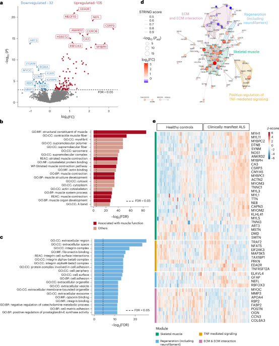
The goal in this step was to select a subset of proteins differentially expressed between clinically manifest ALS and healthy controls (that is, disease state biomarkers) from the ~5,300 in the Olink Explore HT panel for downstream analysis. This step was based on the rationale that proteins differentially expressed between patients with clinically manifest ALS and healthy controls are likely ALS related and would be strong candidates to predict phenoconversion among pathogenic variant carriers. To ensure no overlap between samples used in this step and those used to build prediction models, we included in this step only study participants from the clinically manifest (n = 35) and healthy control (n = 59) groups, each with Olink data from 126 visits (Table 1). As all but 21 controls contributed multiple samples, we employed a mixed-effects model with a random intercept to account for within-person correlation. We also included age at sample collection, sex and genotype group (SOD1 A4V, SOD1 non-A4V, C9orf72 and other pathogenic variants) as covariates. The Benjamini–Hochberg (BH) procedure was applied to control the FDR42 at a significance threshold of 0.05.
Step 1b. Biological implications
Pathway enrichment analysis was performed using the ‘gost’ function in the gprofiler2 package (v0.2.3), which provides functional profiling by mapping differentially expressed proteins to GO, Kyoto Encyclopedia of Genes and Genomes, Reactome and other databases43. Statistical significance was defined as an FDR-adjusted P value (Padj) < 0.05.
Protein–protein interaction (PPI) networks were constructed to investigate the functional connectivity among the differentially expressed proteins. Interactions were queried using the STRING database (v11.5), which integrates evidence from experimental data, computational prediction, co-expression, curated databases and literature mining23. To identify biologically coherent subnetworks, we applied Markov Cluster Algorithm clustering using STRING’s built-in implementation, with an inflation parameter set to 3 to control cluster granularity.
Step 2. Temporal dynamics protein modeling
To evaluate whether the differential abundance observed between patients with clinically manifest ALS and healthy controls can also be detected before phenoconversion, we modeled the longitudinal trajectories of the subset of proteins identified in step 1, using a two-layer GAMM framework44.
Details of the GAMM models are available in Supplementary Information. Briefly, in the first layer, we modeled the protein trajectory in healthy controls only and included sex as a fixed covariate, a random intercept to account for within-participant correlation, and a smooth function of age to capture nonlinear age-related changes in protein abundance. In the second layer, we modeled the relative protein abundance—defined as the deviation from the expected protein abundance in an age- and sex-matched healthy control based on the model in the first layer—over time, including also a random intercept and a smooth function to capture nonlinear protein trajectories. To assess the statistical significance of the disease effect in each model, we applied the BH procedure on smooth terms to control the FDR at a significance threshold of 0.05.
For each protein that exhibited a significant pre-symptomatic change, we determined the earliest time of this change by first constructing the pointwise 95% Bayesian credible interval (CrI) around the fitted curve of the longitudinal protein trajectory, with s.e. values obtained from the Bayesian posterior covariance matrix of the spline coefficients under REML estimation in the mgcv package44; these intervals have good frequentist across-the-function coverage properties45. We then identified the time period(s) during which this CrI excluded 0, indicating a significant difference from age- and sex-matched controls, and considered the start of this period to be the earliest time of pre-symptomatic change (see Supplementary Information for additional details).
In primary analyses, the models included data from both phenoconverters and those with clinically manifest ALS. For the latter group, reported onset of weakness was used as a proxy for phenoconversion. Secondarily, we repeated these models but included only data from phenoconverters (pre-conversion and post-conversion) or only pre-conversion visits from phenoconverters.
Step 3. Time-to-phenoconversion Cox regression
To assess the association between protein biomarker and subsequent phenoconversion, we performed time-to-event analyses using Cox proportional hazards models and baseline protein biomarker data from phenoconverters (that is, those who met phenoconversion endpoint) and pre-symptomatic individuals (that is, those who were censored). We first fitted univariate Cox models, including relative protein abundance as the predictor and adjusting for covariates (age, sex and genotype group). Multiple testing was controlled for using the BH procedure (FDR < 0.05). For multivariable prediction, we constructed partially penalized Cox models with LASSO regularization, penalizing only the protein variables while retaining clinical covariates without penalty. The optimal penalty parameter was selected using leave-one-out crossvalidation. The LASSO-derived risk score for each participant was calculated as a weighted sum of the selected proteins and covariates, using the regression coefficients estimated from the optimal penalized Cox model. The performance of different protein panels was evaluated by comparing those with high versus low risk score (median split) using Kaplan–Meier analysis and log-rank test.
To leverage longitudinal proteomic measurements, we additionally explored univariate and LASSO-penalized, time-dependent Cox models, in which protein abundance was treated as a time-varying covariate updated at each visit. Univariate models were evaluated using the BH procedure with FDR < 0.05 and LASSO penalization was applied to protein variables only, with clinical covariates retained unpenalized and the optimal penalty parameter selected by leave-one-out crossvalidation.
Step 4. Phenoconversion event prediction
Using the differentially expressed proteins (that is, disease state biomarkers) identified in step 1, this step aimed to build prediction models for whether a pre-symptomatic pathogenic variant carrier will phenoconvert to ALS within a certain timeframe (T), with T ranging from 0.5 years to 5 years. To enhance model robustness, we used absolute protein levels (NPX) rather than relative protein abundance in these prediction models. This choice eliminates the dependence on a reference control population for calibration and ensures applicability in clinical settings where repeated measurements or a similar control reference may not be available. Training data were drawn from the pre-symptomatic and phenoconverter groups, with each visit annotated as either ‘case’ or ‘control’, depending on, respectively, whether or not phenoconversion occurred within the specified time period after the visit. For the pre-symptomatic group, all visits with subsequent follow-up time longer than (or equal to) T were annotated as ‘controls’; the remaining visits were excluded because we do not know whether the participant might still phenoconvert within the T-year interval. For the phenoconverter group, all visits where phenoconversion occurred more than T years after the visit were considered to be ‘controls’, whereas all visits where phenoconversion occurred within T years of the visit were considered to be ‘cases’. Each phenoconverter’s first post-conversion visit was also included and labeled as a ‘case’, whereas all other post-conversion visits were excluded.
We evaluated seven machine learning approaches and decided on LR, with fivefold crossvalidation for model training and testing (see Supplementary Information for additional details).
We tested five different timeframes: T = 0.5, 1, 2, 3 and 5 years. For each timeframe, we first ran univariate LR for each protein individually, with covariates for sex, age (at sample collection) and genotype group. From the results, we identified the proteins that returned the best prediction measured by AUC of a ROC curve. Next, we performed a greedy stepwise LR with forward greedy search. Specifically, we progressively added, one at a time, proteins that maximized the incremental (or minimized the decremental) predictive performance among all remaining proteins. Performance was measured using the average AUC across the fivefold crossvalidation. The model with the best predictive performance in the testing set was selected as the designated model for that timeframe. We counted how many times each of the differentially expressed proteins from step 1 are included in the five designated models (one for each timeframe). Among the proteins that appeared at least once in the five models (Extended Data Table 3), we further filtered them based on their ranking, the timeframe(s) in which they appeared, as well as biological rationale to arrive at a small core panel of proteins as susceptibility/risk biomarkers (see Supplementary Information for additional details).
Similarly, and in parallel, we undertook a purely data-driven approach (that is, without expert curation), using greedy forward selection to identify a small panel of proteins that predicted phenoconversion across the different timeframes, based on their average crossvalidation AUCs across these timeframes.
To determine the optimal classification threshold of the resulting core protein panels, we used Youden’s index derived from the ROC curve. Specifically, for each model we identified the threshold that maximized Youden’s J statistic (sensitivity + specificity − 1), which represents the point that optimally balances sensitivity and specificity. This threshold was then used to predict whether an individual would phenoconvert within T years after the visit, classifying each individual as either a converter or a nonconverter.
To illustrate the association between the baseline risk score of multi-protein panels and phenoconversion-free survival, we employed partially penalized LASSO Cox analysis, as well as Kaplan–Meier analysis and log-rank test, as described in step 3 above.
Step 5. Phenoconversion timing estimation
Our goal in this step was to build disease progression models to estimate pre-symptomatic mutation carriers’ proximity to time of phenoconversion given the proteomic profile obtained from the individual’s most recent visit and baseline visit, similar to the approach employed in a recent study of familial FTD that utilized a Bayesian disease progression model17. For this step, we used the final protein panel identified in step 4. Instead of LR, we used a truncated regression model and included only data from the pre-conversion visits of phenoconverters, the only group in whom time to phenoconversion is known. To avoid the collinearity between age and time to phenoconversion, we used relative protein abundance from step 2 as input features. Given the longitudinal structure of the proteomics data, with repeated measurements collected from the same individuals over time, we used each participant’s baseline visit as an internal reference to account for interindividual variability in protein abundance. To model time to phenoconversion as a continuous outcome, we employed truncated regression and included sex and genotype group as covariates (see Supplementary Information for additional details).
The predicted and observed time to phenoconversions were compared and summarized using the RMSE, MAE and Pearson’s correlation. The performance of the multi-protein panel model was compared to the NEFL-only model using the likelihood ratio test to determine whether the multi-protein panel provided a significant improvement in phenoconversion timing estimation above and beyond NEFL.
UKB replication
For replication analysis, we used data from the UK Biobank (UKB) cohort. UKB is a large-scale prospective study that recruited 503,317 participants aged 40–69 years between 2006 and 2010 across the UK19,46, with Olink Explore 3072 data available through the UKB-PPP for n = 54,21947. Data for the present analysis were accessed under application no. 847687.
The replication cohort consists of five participant groups (Table 1), four of which are similarly defined as in the discovery cohort: heathy control, pre-symptomatic, phenoconverter and clinically manifest. A fifth group (pre-hospitalization) was also included in the modeling of protein trajectories (see Supplementary Information for detailed description of the inclusion and exclusion criteria for each group).
From among the UKB-PPP participants, because we need genotype information to determine eligibility for the control versus the pre-symptomatic group, as well as to adjust for genotype in replication analyses (as is done in discovery analyses), we included only the n = 52,488 for whom whole-genome sequencing data were also available and who had neither withdrawn consent nor been lost to follow-up (datafield 190 in UKB), as of the time of data access in August 2025 (Extended Data Fig. 5).
For replication analysis, we applied the differential protein expression approach (as described in step 1 above) to the UKB-PPP cohort, using covariate-matched healthy controls for individuals in the clinically manifest group, with covariates including sex, age and genotype group. Of the 137 proteins identified in the discovery cohort, 95 were available in the UKB due to differences between the Olink Explore 3072 and the Olink Explore HT platforms. We plotted the log2(FC) of the overlapping proteins and assessed the correlation between discovery and replication cohorts via Pearson’s correlation. To analyze the temporal dynamics of proteins in the replication cohort, we applied two-layer GAMs instead of two-layer GAMMs, because the UKB data were cross-sectional rather than longitudinal. Accordingly, individual-level random effects were excluded from the models. In the first-layer GAM, relative protein abundance was modeled with a covariate sex and a smooth term of age. The second-layer GAM modeled relative protein abundance against a smooth term of proxy for time to phenoconversion. We then tested our phenoconversion timing estimation models trained on the discovery cohort to baseline protein expression levels in the replication cohort, with covariates including sex, age and genotype group.
Reporting summary
Further information on research design is available in the Nature Portfolio Reporting Summary linked to this article.