Health system learning enables generalist neuroimaging models

Health system learning

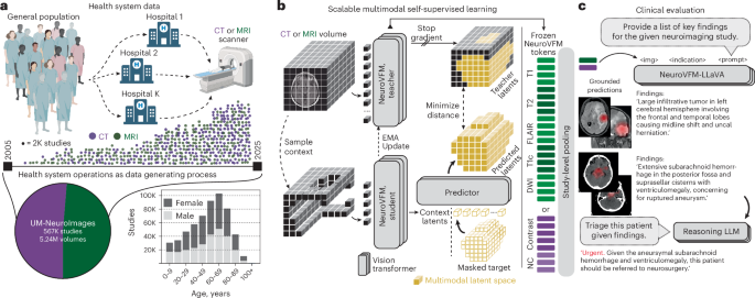
We define ‘health system learning’ as learning directly from uncurated data generated during routine clinical operations. This is distinguished from internet-scale pretraining, which lacks access to private clinical data, and from report-supervised health system pretraining, which is bottlenecked by requiring paired reports and what they capture. Health system learning can also be contrasted with standard machine learning pipelines that include data selection for a specific disease—for example, brain tumor MRIs or patients with Alzheimerʼs disease—and subsequently training a classifier to diagnose that disease. Health system learners are trained without a specific diagnosis or classification as a target. We also clarify that health system learning does not imply learning from ‘all data’ within a health system. Rather, health system learning is the environment within which generalist medical foundation models can emerge²⁹. We introduce NeuroVFM as the imaging-first instantiation of this approach on clinical neuroimaging CT and MRI scans.

UM-NeuroImages dataset

Radiology studies at large academic medical centers are stored in picture archiving and communication systems (PACSs). We queried the University of Michigan PACS via an SQL-based interface (Sectra Data Warehouse (SDW)) for neuroimaging studies satisfying three criteria: (1) acquisition data prior to 1 June 2024; (2) an examination of body part(s) including the head, brain, orbits, face or neck; and (3) a modality of MRI or CT. The specific query parameters are in Supplementary Fig. 5.

The initial query yielded 645,989 unique studies. We excluded 79,074 entries that contained non-image objects (for example, PDFs and screenshots) or corrupted Digital Imaging and Communications in Medicine (DICOM) files. The final cohort comprised 566,915 studies (275,981 MRI; 290,934 CT) totaling 5,239,579 series (3,647,950 MRI; 1,591,629 CT). We split the data temporally: studies acquired before 1 June 2023 formed the training set, and studies from 1 June 2023 through 31 May 2024 formed the test cohort. We only included studies with reports for the test set, resulting in 21,054 CT studies and 29,239 MRI studies. The full training set was used for self-supervised pretraining of the NeuroVFM encoder, which requires no labels or reports. All downstream supervised evaluations used the 444,188 training studies with paired radiology reports (219,882 MRI; 224,306 CT). From this report-paired subset, we held out 991 MRI studies and 722 CT studies as a validation set for hyperparameter tuning.

Labels were derived from radiology reports using an LLM-based extraction pipeline, and a stratified subset was manually reviewed by clinical experts. We first define a clinically organized ontology of 82 CT and 74 MRI diagnoses (Extended Data Fig. 2h). We then used GPT-4.1-mini to extract these 156 diagnoses from radiology reports and to generate structured summaries of key findings, following previous report-parsing work^13,30,31,32. Prompts used are in Supplementary Figs. 6−8. To assess annotation quality, two neuroimaging experts (R.J. and T.H.) independently reviewed a stratified sample drawn across all diagnostic labels. For each label, we selected two pipeline-positive and two pipeline-negative studies, providing the label, report text and clinical indication. Reviewers were blinded to pipeline predictions and determined whether the label was supported by the accompanying report and indication. Annotation performance metrics are reported in Supplementary Table 1.

Series preprocessing

To ingest the full breadth of health system data without manual curation, we applied an automated pipeline to standardize intensities and dimensions. Series were resampled to 1 × 1 × 4 mm (4 mm along the acquisition axis from DICOM) and saved as an 8-bit uint. MRI intensities were clipped to the 0.5−99.5th percentile before quantization. CT volumes yielded three windows: brain (width = 80, level = 40; 8-bit), subdural/blood (width = 200, level = 80; 4-bit) and bone (width = 2,800, level = 600; 4-bit). The 4-bit windows reduced storage while preserving contrast for key pathologies. Background masks were derived via Otsu and Hounsfield thresholding for MRI and CT, respectively. During training, volumes were cast to float32, scaled to [0,1] and mean normalized using statistics derived from the training set. Extended Data Fig. 1b summarizes this pipeline.

NeuroVFM training with Vol-JEPA

The core training objective for NeuroVFM was large-scale self-supervision, applied at the individual volume level, across the entire UM-NeuroImages dataset. NeuroVFM employs a JEPA to optimize a masked modeling objective directly in the representation space. First, input volumes are tokenized into non-overlapping 3D patches of 4 × 16 × 16 voxels. Each 3D volume is then partitioned into a small, visible context region, x, and a larger, masked target region, y. The tokenized context region is processed by a trainable student encoder, E_θ. The resulting context representations, E_θ(x), along with positional information of the masked target patches, are then fed to a predictor module, P_ϕ, which generates predictions for the representations of these target patches. The complete set of tokens from the input volume (representing both context and target regions) is processed by a teacher encoder, whose weights, \({E}_{\bar{\theta }}\), are updated as an exponential moving average (EMA) of the student encoderʼs weights after each step and are not directly optimized by gradient descent. The training objective minimizes the difference between the predicted representations of the target patches and those generated by the teacher network for the same target patches. This is formulated as⁵:

where Δ_y is a set of learnable tokens that represents the masked target patches, and sg( ⋅ ) denotes a stop-gradient operation. This representation-level objective is computationally efficient and encourages the learning of semantic features without requiring explicit voxel-level augmentations or decoding.

Vol-JEPA extends the principles of I-JEPA⁵ and V-JEPA⁷ for self-supervision to volumetric neuroimages, predicting representations of masked 3D target patches based on visible 3D context patches. This encourages the model to learn the shared anatomy of the brain, head and neck. The masking strategy was foreground focused: context and target patches were sampled exclusively from the precomputed head mask. Masking was performed in two ways: (1) multiple large crops are sampled, with their union forming the masked target, and (2) a small crop is sampled as context, with the complement being the target. A random subset of context patches is then dropped, serving as additional target patches to predict. Unlike approaches that truncate sequences within a mini-batch to a uniform length, our implementation leverages FlashAttention-2 (ref. ³³) to directly encode variable-length sequences of context and target patches derived from input volumes. To ensure robustness to varying patient orientations, we applied random axis permutations and flips to each volume, using the same transform for both student and teacher inputs. A hyperparameter search indicated optimal context region sampling ratios (from the total patches within a given crop) are 25% for MRI volumes and 20% for CT volumes, with a patch dropout rate of 20%. An overview of this masking strategy can be found in Extended Data Fig. 3a.

During training, volumes were truncated along each axis to a maximum of 20 patches to bound the token count per crop. At inference, the same encoder was applied to the entire volume without truncation, leveraging its ability to handle variable-length token sequences. For CT scans, which are typically viewed with multiple windowing presets (for example, brain, subdural and bone), we implemented a weighted sampling strategy during training. For pretraining, one of these three CT window settings was randomly selected and applied with probabilities of 0.7 (brain), 0.15 (subdural) and 0.15 (bone), and all windows were used during inference. Full training details are in Supplementary Table 9.

Grounded diagnoses with multiple instance learning

Most visual grounding evaluation requires an object detection module to output a bounding box around an image region given a label or text prompt. This is not feasible for the present study because there are no object detection datasets or models sufficiently powerful to evaluate neuroimage grounding on the scale and complexity of UM-NeuroImages. Because most neurologic pathologies are spatially small relative to the full study, study-level labels provide only weak supervision. We leveraged an attention-based multiple instance learning (AB-MIL) framework to assess neuroimage grounding³⁴. AB-MIL is known to assign high attention to diagnostic regions in medical images³⁵. Unfortunately, the standard AB-MIL framework, with its ‘aggregate-then-classify’ design, cannot resolve a critical grounding ambiguity: it is unable to disentangle a patch’s importance (‘where’ the model looks) from its directional contribution (‘why’ it is considered positive or negative evidence).

We address this gap with a pooling operation that reverses the standard order to a ‘classify-then-aggregate’ model. For a task with K classes and a bag of N instances, we first compute classification logits for each instance i using a multilayer perceptron (MLP), ψ_p. A separate attention MLP, ψ_m, generates K class-specific attention scores per instance. For each class, these scores are normalized with a softmax across instances to obtain class-specific attention weights. The final bag-level logits, p(x), are the sum of the elementwise product of the per-instance logits and their corresponding attention weights:

Here, f(x_i) is the frozen feature vector for instance i; α_i is the vector of class-specific attention weights; and ∘ denotes the Hadamard product. This formulation yields interpretable, label-specific attention maps that reflect both the importance and directional contribution of each region to the diagnostic decision, providing a scalable means of evaluating grounding without region-level annotations.

Comparison to foundation model baselines

We evaluated NeuroVFM against two families of baselines: (1) internet-scale pretrained encoders and (2) methods directly trained on UM-NeuroImages. All backbones were frozen and evaluated with the same study-level attentive probe and data splits. Full architecture details, training hyperparameters and evaluation configurations can be found in Supplementary Table 9 and in our GitHub repository. A schematic of the study-level pooling strategies can be found in Extended Data Fig. 1e.

Internet-scale pretrained encoders

We chose two baselines representative of the dominant internet-scale paradigms:

For CT studies, all baselines were provided the same set of windowed series as NeuroVFM (with brain, blood and bone windows given as separate series). 3D volumes were processed slicewise according to the modelʼs respective preprocessing pipeline (for example, DINOv3 necessitates resizing to 224 × 224 and normalizing with ImageNet mean/s.d.), with slice-level features aggregated to produce study-level predictions.

Methods trained on UM-NeuroImages

To isolate the effect of pretraining objective from data, we trained several baseline architectures on UM-NeuroImages spanning the following paradigms: voxel reconstruction (MAE-style), self-distillation (DINO-style) and study report alignment (CLIP-style). For voxel reconstruction, we trained NeuroMAE, which uses the same 3D ViT encoder, pretraining data and optimization schedule as NeuroVFM but replaces the latent prediction objective with voxel reconstruction³⁶. We adjusted the decoder size and masking ratio, using 85% foreground-masking random masking. This pairing directly isolates the effect of the pretraining objective. For self-distillation, we trained a DINOv2 model¹¹ on two-dimensional (2D) slices derived from UM-NeuroImages volumes. For report-supervised pretraining, we trained HLIP⁸, a 3D medical vision-language model, on 444,188 study−report pairs from UM-NeuroImages and evaluated its frozen image encoder. HLIP training mini-batches were balanced across MRI and CT studies, and the CLIP objective was computed within each modality to prevent trivial cross-modality discrimination. We additionally benchmarked PRIMA⁴, a 3D vision-language model trained on the MRI subset of UM-NeuroImages, as a second report-supervised baseline.

Diagnostic evaluation of NeuroVFM

The UM-NeuroImages dataset contains two decades of clinical neuroimaging data from a large academic health system, spanning a broad spectrum of neurological presentations. To evaluate ‘imaging-only’ diagnostic ability, we tested NeuroVFM on a temporally held-out test cohort beginning immediately after the pretraining window. All encoders were frozen, and modality-specific attentive probes were trained for multi-label prediction using class-weighted binary cross-entropy. We prespecified a primary endpoint of macro-averaged AUROC across all 156 diagnostic tasks and a secondary endpoint of per-category AUROC. For the primary endpoint, pairwise differences between models were assessed by paired, study-level bootstrap (10,000 replicates). For the secondary endpoint, category-level comparisons were corrected for multiple hypotheses using Benjamini−Hochberg correction at q < 0.05. Hyperparameters and class-specific thresholds were selected on the validation set. We report per-class AUROC, balanced accuracy, sensitivity and specificity on the test cohort, with 95% CIs from study-level bootstrap resampling. Full results are provided in Supplementary Tables 10 and 11.

Because the split is temporal rather than patient level, patients who received imaging in both periods appear in both training and test sets (34.7% of MRI and 31.8% of CT test set patients). This mirrors the intended deployment setting, where a model trained on historical data encounters both new and returning patients. To verify that this overlap does not inflate performance, we repeated all evaluations after removing studies from overlapping patients. Aggregate performance and model rankings were largely unchanged (Supplementary Table 12).

Data, model and modality scaling

We studied performance along data scale, model capacity and modality with resource-normalized protocols. For modality, we held the optimization budget fixed at approximately 510,000 training steps and compared (1) a single multimodal model versus (2) two unimodal models (one MRI, one CT) trained separately. For data and model scaling, we varied (1) the fraction of UM-NeuroImages (5%, 10%, 25%) and (2) the encoder size (ViT-Small, ViT-Medium, ViT-Base). Larger backbones (for example, ViT-Large) were left to future work due to computationally prohibitive hyperparameter search.

Label efficiency

We quantified how per-task performance scales with the amount of supervision. For each diagnostic class c and modality m ∈ {CT, MRI}, we calibrated model probabilities on the validation set using Platt scaling and computed F1 on the held-out test set. We excluded classes with fewer than 30 training positives (n_pos) and 10 testing positives. We fit a simple linear model of F1 versus \({\log }_{10}({n}_{{\rm{pos}}})\) via ordinary least squares (OLS) with heteroskedasticity-consistent standard errors of type 3 (HC3 SEs). Modality fixed effects and interactions assessed CT versus MRI differences. Encoder comparisons (NeuroVFM versus HLIP, DINOv3 and BiomedCLIP) used ANCOVA to test slope equality. If interaction terms were non-significant, a shared slope was used; otherwise, encoder-specific slopes were retained. Label equivalence was reported as the fold increase in positives that a baseline requires to match NeuroVFM at a fixed F1, with 95% CIs from 10,000 bootstrap replicates over classes.

NeuroVFM on external public benchmarks

To assess out-of-distribution generalization, we evaluated frozen NeuroVFM performance on eight public neuroimaging benchmarks. For all tasks, we trained an attentive probe without updating the encoder. Within each dataset, we held out 20% of patients as a stratified test set. On the remaining 80%, we performed eight-fold iterative stratified cross-validation to select probe hyperparameters. The eight probes trained on the cross-validation folds were then used to generate logits on the held-out test set, which were averaged per study to form the final ensemble. All reported metrics include 95% study-level boostrapped CIs (10,000 replicates). This approach rigorously tests the quality of the learned representations and, through the probeʼs attention weights, allows for the identification of class-discriminative tokens for each task.

External MRI benchmarks

We evaluated NeuroVFM on six public MRI datasets, spanning a range of neurological and psychiatric conditions. On the multi-site OpenBHB dataset³⁷, we benchmarked brain age regression to test for fine-grained anatomical representation. For dementia-related tasks, we used the ADNI dataset³⁸ to perform cognitively normal versus Alzheimerʼs disease classification and to distinguish progressive from stable mild cognitive impairment (sMCI versus pMCI), with a 20% stratified test set held out within ADNI. We then evaluated the ADNI-trained Alzheimerʼs disease classifier externally on the OASIS-1 (ref. ³⁹) and AIBL⁴⁰ datasets, applying the frozen probe without further fine-tuning to distinguish cognitively normal individuals (Clinical Dementia Rating (CDR) = 0) from those with dementia (CDR ≥ 1). We further evaluated diagnostic classification on several consortium datasets: differentiating individuals with autism spectrum disorder from typically developing controls on the ABIDE dataset⁴¹ and Parkinsonʼs disease from healthy controls on the PPMI dataset⁴².

External CT benchmarks

Performance on detecting critical neuroradiological findings was evaluated on two public non-contrast head CT cohorts, selected to test generalization on both a large-scale challenge dataset and a smaller, deeply annotated clinical cohort. The large-scale 2019 RSNA-ICH challenge dataset⁴³ was used to benchmark multi-label classification of intracranial hemorrhage and its five subtypes (epidural, intraparenchymal, intraventricular, subarachnoid and subdural). The high-quality, expert-annotated CQ500 dataset⁴⁴ was used for a more extensive evaluation across 14 diagnostic labels, including detailed hemorrhage characterization (subtypes, laterality, chronicity), skull fracture detection and signs of structural abnormality (for example, mass effect and midline shift).

Vision instruction tuning for radiology report generation

To evaluate the potential of NeuroVFM as a visual backbone for multimodal applications, we adapted a LLaVA-1.5-style visual instruction tuning framework¹⁶. This experiment was designed not to optimize report generation performance but, rather, to assess the feasibility of coupling NeuroVFMʼs learned representations with an LLM with minimal architectural modifications.

NeuroVFM-LLaVA architecture

NeuroVFM-LLaVA comprises three components: (1) the frozen NeuroVFM visual encoder, (2) an open-source LLM (Qwen3-14B)¹⁵ and (3) a connector module to bridge them.

Standard LLaVA connectors use a two-layer MLP to project visual features into the LLMʼs word embedding space. This approach is insufficient for the high dimensionality of multi-sequence neuroimaging, where a single study may comprise a large and variable number of visual tokens (≥20,000). To address this, our connector module first employs a Perceiver-style architecture that operates sequencewise (for example, on T1, T2 and FLAIR independently)^45,46. The Perceiver aggregates the variable-length token sequence from each scan into a fixed-length representation of 64 latents. These fixed-length latents (total latents = 64× num_sequences) are then concatenated and passed to a two-layer MLP projector.

Training dataset and curation

The training dataset was derived from 444,188 unique neuroimaging studies. To create the text pairs, original radiology reports were summarized using GPT-4.1-mini to extract a concise list of key radiological findings.

Acknowledging that naive training on imbalanced medical datasets can degrade performance, we curated the training set via data resampling. Using the previously extracted diagnostic labels from each report, we performed weighted random sampling with replacement, assigning each study a weight inversely proportional to the prevalence of its rarest associated label. This process, which aims to balance the representation of less common pathologies, resulted in the final training dataset of approximately 270,000 unique image−text pairs (444,188 total including duplicates).

Training strategy

Following the LLaVA methodology, training proceeded in two stages.

1. 1.

   Stage 1 (Connector Pretraining). Only the connector module (Perceiver and MLP) weights are updated. The model was trained to map NeuroVFM image features to the corresponding reference key findings, which were formatted as a single, concatenated string.

2. 2.

   Stage 2 (Full Fine-tuning). Both the connector and the LLM weights are updated. In this stage, the model was trained on an instruction-following task. The input prompt was fixed to: ‘Generate a concise report of the key positive findings for this study.’ The target output was the same set of findings but formatted as a structured JSON list ordered by clinical relevance.

Further details on training hyperparameters are provided in Supplementary Table 13.

Evaluation of preliminary report generation

We evaluated NeuroVFM-LLaVA against two proprietary multimodal frontier models: GPT-5 (gpt-5-2025-08-07, ‘reasoning’ medium, ‘verbosity’ low) and Claude Sonnet 4.5 (claude-sonnet-4-5-20250929, ‘thinking’ enabled). We additionally evaluated MedGemma 1.5 4B, an open-source healthcare MLLM by Google DeepMind. This evaluation assessed two criteria: (1) the factual accuracy of generated findings and (2) the clinical utility of these findings for a downstream triage task. To support this evaluation, we established business associate agreements (BAAs) with vendors offering commercially available Health Insurance Portability and Accountability Act (HIPAA)-compliant access to frontier models, specifically OpenAI and Anthropic. This enabled the secure exchange of protected health information (PHI) while preserving patient privacy. The prompt used to generate study findings using frontier models can be found in Supplementary Fig. 9.

Benchmark model adaptation (3D-to-2D conversion)

A primary challenge in benchmarking against proprietary models is that they accept only 2D images and have limitations on total input image tokens. To create a fair comparison with our 3D-native model, we developed a systematic 3D-to-2D conversion pipeline.

1. 1.

   All 3D volumes (preprocessed with the NeuroVFM pipeline) were converted into 224 × 224-pixel 2D slices by resampling along the axis of acquisition and keeping every other slice. For MedGemma 1.5, CT studies were processed as three-channel 2D slices with each channel representing a different windowing, as per their specifications⁴⁷.

2. 2.

   Non-diagnostic and derived sequences (for example, scout images and phase/magnitude maps) were excluded.

3. 3.

   Due to application programming interface (API) token limits, inputs were constrained to 15 sequences per study for GPT-5 (approximately 360 slices) and four for Claude Sonnet 4.5 (approximately 96 slices). For MedGemma 1.5, we provided two sequences per study as we found that led to optimal performance.

4. 4.

   If a study exceeded this limit, sequences were deterministically prioritized based on clinical relevance (that is, for MRI: post-contrast T1, diffusion-weighted imaging/apparent diffusion coefficient (DWI/ADC), FLAIR, susceptibility-weighted imaging (SWI), T2, non-contrast T1; for CT: at least one brain, blood and bone window).

5. 5.

   All selected slices were converted to float and normalized between [0,1], and slices with more than 90% black pixels were dropped.

Increasing from five to 15 series per study improved three-tier acuity accuracy only marginally on both MRI and CT, indicating that performance differences between models were not driven by input volume (Extended Data Fig. 9e).

Expert evaluation of generated reports

All generative models were evaluated on ‘UM-NeuroImages-Acuity’, a new, manually curated test set of 600 studies (300 validation, 300 hold-out) derived from our test set. This set was hand-selected by neuroimaging experts to be balanced across three acuity classes (‘Unremarkable’, ‘Routine’, ‘Urgent’) and two modalities (MRI, CT). This allows for estimation of class-conditional safety metrics rather than prevalence-weighted deployment performance.

We assessed report quality through automated metrics, BLEU-2 (ref. ⁴⁸), ROUGE-L⁴⁹ and METEOR⁵⁰, as well as with human evaluation. To ensure effective blinding, all model outputs were standardized to a uniform text format. For NeuroVFM-LLaVA and GPT-5, a neuroimaging expert (T.H.) performed a structured review of each study to quantify (1) capture of key findings, (2) clinically significant hallucinations and (3) laterality errors. To evaluate preferences, three neuroimaging experts from the United States and Europe (R.J., A.-K.M. and T.H.) then performed a blinded, randomized pairwise review comparing generated findings from NeuroVFM-LLaVA and GPT-5 against the ground truth clinical report. For each case, model outputs were randomly labeled ‘Report A’ and ‘Report B’. Evaluators selected their preferred report (‘Report A’, ‘Report B’ or ‘Both’) based on overall clinical utility for acuity assessment. Because Claude Sonnet 4.5 and MedGemma 1.5 both exhibited substantially lower acuity accuracy on UM-NeuroImages-Triage, we restricted expert review and preference testing to NeuroVFM-LLaVA and the strongest baseline (GPT-5).

To quantify the clinical utility of the generated findings, we employed an ‘LLM-as-a-judge’ pipeline. In each analysis, we designated a frontier model (GPT-5 or Claude Sonnet 4.5) as a separate ‘acuity assessor’, instructed with a strict, predefined set of criteria (Supplementary Fig. 1). We first confirmed that each LLM achieved high accuracy when classifying acuity from the ground truth radiology report alone. The LLM was then prompted to classify each study as ‘Unremarkable’, ‘Routine’ or ‘Urgent’ based solely on the generated text findings from each model (NeuroVFM-LLaVA, GPT-5 and Claude Sonnet 4.5) and the clinical indication. Using GPT-5 versus Claude Sonnet 4.5 as the acuity assessor yielded similar results, indicating that the protocol is model agnostic and not biased toward any single frontier model. This procedure converts report generation into a three-class classification problem and provides a quantitative measure of clinical utility.

Prospective feasibility study of report sufficiency for triage

We conducted a prospective silent evaluation over a consecutive 1-week window (18−25 January 2026), including all CT and MRI studies of the head, brain, face, neck and orbits performed during routine care (n = 1,155; 601 MRIs and 544 CTs). No additional curation or exclusion criteria were applied beyond modality and anatomic region. For each study, we generated a structured report using (1) NeuroVFM-LLaVA or (2) GPT-5, a multimodal baseline demonstrated to be the best model at findings generation in Fig. 4. Reviewers were blinded to the source of the report (ground truth, NeuroVFM, GPT-5) when evaluating.

To approximate a workload-aware triage workflow, we used a fixed two-stage process. First, a frontier reasoning model (GPT-5-thinking with a prespecified prompt and temperature) screened each report and assigned a binary decision: ‘flag for clinician review’ or ‘do not flag’. Second, for all flagged studies, a panel of imaging-centric clinicians assigned a final, gold standard triage label (urgent versus non-urgent) based solely on the model-generated report and clinical indication. Specifically, two clinicians (T.H. and A.P.) independently annotated flagged studies, and the third expert (R.J.) adjudicated any discordant labels. Urgent cases were defined as studies containing findings that would reasonably warrant escalation or intervention. To assess whether the screening step was failing to capture urgent studies, we additionally audited all unflagged studies, with all but one being non-urgent (99.9% sensitivity). This study was moved into the flagged subset for final evaluation. Each study was assigned a reference urgency label derived from the ground truth radiology report.

The primary analysis evaluated whether generated reports were sufficient to support accurate triage under the two-stage workflow. We quantified (1) the fraction of studies flagged for review (workload proxy), (2) urgent miss rate attributable to the screening stage (urgent studies not flagged), (3) triage performance among flagged studies and (4) overall triage performance (balanced accuracy and urgent miss rate). For each metric, we computed 95% CIs using study-level bootstrapping (10,000 replicates).

Computational hardware and software

All data used to train NeuroVFM were acquired over more than two decades of routine clinical care at Michigan Medicine. Studies were identified in the Michigan Medicine PACS via the SDW. The aggregate size of raw Neuroimaging Informatics Technology Initiative (NIfTI) volumes is approximately 150 TB, stored on the Advanced Research Computing (ARC) DataDen object storage service. Postprocessing (removal of non-image/corrupt entries and embedded metadata, background removal and quantization) reduced the footprint by over an order of magnitude to approximately 9 TB. Preprocessed volumes were written as large NumPy memory-mapped shards (10 shards for the training set; one each for the validation and test sets) with JSON index manifests to enable zero-copy random access during training.

All experiments were executed on the University of Michigan ARC Armis2 cluster using Simple Linux Utility for Resource Management (SLURM). Typical jobs used nodes with eight NVIDIA L40S GPUs (48 GB each), 64 Intel Xeon Platinum 8358 CPU cores and 503 GB RAM. Vol-JEPA pretraining used PyTorch Distributed Data Parallel (DDP), whereas LLM fine-tuning used PyTorch Fully Sharded Data Parallel (FSDP). A full Vol-JEPA pretraining run required fewer than 1,000 GPU hours in aggregate (batch size of 768, approximtely 510,000 steps), making the approach feasible on university-hosted compute clusters. Training used automatic mixed precision (AMP) with fixed random seeds.

For single-volume inference in bfloat16, peak GPU memory ranges from 0.89 GB (ViT-Small, 21.7 million parameters) to 1.10 GB (ViT-Base, 85.8 million parameters) on a single L40S, with throughput of 84 volumes per second across all encoder sizes. Models were implemented in Python 3.10.14 with PyTorch 2.5.0 (CUDA 12.4). Vol-JEPA pretraining and diagnostic probing used PyTorch Lightning 2.5.0.post0. All data handling and computation occurred on HIPAA-compliant ARC infrastructure. Model weights are available under the CC-BY-NC-SA-4.0 license, enabling the broad dissemination of learned clinical representations without the risk of PHI leakage.

Use of LLMs

LLMs were used to assist with code prototyping and manuscript editing. All analyses, text and code were reviewed and verified by the authors, who take full responsibility for the work.

Ethical, regulatory, governance and inclusion statement

Our research was approved by the University of Michigan institutional review board (IRB) (HUM00229133). All MRI and CT data were acquired under secondary data usage. The methods were carried out in accordance with the IRBʼs guidelines, regulations and policies. All human subjects who met inclusion criteria as stated above were included in the study. No treatment decisions were informed by NeuroVFM, as our model is not approved by the US Food and Drug Administration. Our model is susceptible to bias secondary to training dataset, model architecture and objective functions. NeuroVFM should be used as a research tool only.

Reporting summary

Further information on research design is available in the Nature Portfolio Reporting Summary linked to this article.