
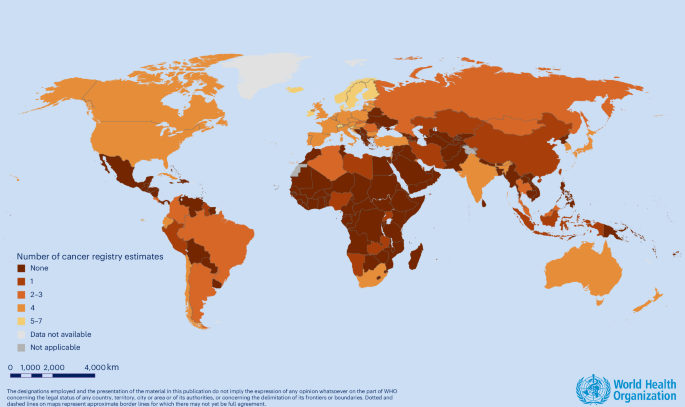
To predict 5-year net survival for women diagnosed with breast cancer between 2017 and 2021 for all countries, a Bayesian hierarchical statistical model was used to combine information from PBCR estimates, covariates plausibly associated with breast cancer survival, and regional levels and trends. Cancer registry survival estimates were obtained from global and regional studies. Cancer registry estimates from 1995 onward were incorporated to maximize geographic coverage and gain insights into temporal trends. Covariate information, including socioeconomic, general healthcare access, and cancer-specific care and outcome indicators, were extracted from systematic reviews, surveys and publicly available datasets (Extended Data Tables 2 and 3).
Data sources for survival
CONCORD-3, the third iteration of the CONCORD study, collected individual-level data on more than 6 million breast cancer diagnoses from 2000 to 201415. Data for 41 countries covered 100% of the national population. In our study, survival predictions were primarily based on CONCORD-3 estimates, supplemented by CONCORD-2 data to either extend the time series between 1995 and 1999 for countries included in CONCORD-3, or provide data between 1995 and 2009 for countries not included in CONCORD-315,54.
Additional estimates from the SURVCAN-3 and NORDCAN studies were also used to complement CONCORD survival estimates. SURVCAN-3 included around 200,000 breast cancer diagnoses during 2008–2012 in 32 countries across Africa, Central and South American, and Asia14. NORDCAN included over 700,000 women diagnosed with breast cancer during 1977–2023 in six Nordic countries55.
All three studies provided net survival estimates; no patient-level data were used. Net survival measures the probability of surviving cancer itself, after removing the influence of other causes of death (background mortality)56. Rather than relying on cause-of-death information, which is not recorded consistently enough for reliable international comparisons57, net survival adjusts for background mortality using life tables.
Survival estimates from CONCORD and SURVCAN-3, or NORDCAN, were considered comparable because they used similar methods to estimate survival. More specifically, in both SURVCAN-3 and NORDCAN, survival was calculated using the nonparametric Pohar Perme estimator and survival values were age-standardized using the International Cancer Survival Standards group 1 weights, for cancer types with a steeply increasing age distribution56,58. Only NORDCAN adopted adjusted age bands, but following the same age dependency of International Cancer Survival Standards cluster 1.
CONCORD considered survival estimates less reliable if they were derived from cancer registries with 15% or more of patients subjected to any of the following criteria: (1) missing or incomplete dates, (2) identified only through a death certificate or autopsy, or (3) lost to follow-up or recorded as alive but censored within 5 years15. In this analysis, all survival estimates with possible reliability issues were excluded. The same cutoffs used by the CONCORD program were used for all data sources.
Population-based survival estimates are the most reliable way to assess how effectively a healthcare system manages patients with cancer because they include all diagnosed cases within a country or territory. Conversely, hospital-based survival estimates can be valuable where PBCRs do not exist or where their survival estimates include a very high percentage of losses to follow-up. To maximize both the use of available survival data and geographical coverage, we incorporated hospital-based survival estimates from the African Breast Cancer-Disparities in Outcomes (ABC-DO) prospective study, but only for countries or calendar periods not covered by CONCORD. ABC-DO presented 5-year, net survival estimates for 2,228 women diagnosed with breast cancer across five sub-Saharan countries between 2014 and 201759. Only for ABC-DO did we use unstandardized survival estimates given the high proportions of young women with poor outcomes in these countries.
In summary, the main data sources were the CONCORD-2 and CONCORD-3 studies (diagnoses 1995–2014), supplemented by SURVCAN-3 for Bahrain, Setif and Batna in Algeria, and Golestan in Iran. NORDCAN estimates for diagnoses from 1989 to 2023 were preferred over CONCORD estimates for six Nordic countries—Denmark, Finland, Iceland, Norway, Sweden, the Faroe Islands and Greenland—as survival time points were more granular in NORDCAN. Hospital-based ABC-DO estimates (2014–2017) were used for Namibia, Nigeria, Uganda, Zambia, and Eastern Cape in South Africa.
Country consultation
The preliminary WHO survival estimates were submitted to countries for consultation. This process aimed at ensuring transparency by enabling countries to review their own preliminary survival estimates, provide technical feedback based on available national data, and submit any additional information on survival or stage distribution. Any data submitted during the country consultation had to comply with strict methodological requirements specified in a data template, such as calendar periods of interest, data quality constraints and proper accounting of background mortality in the derivation of net survival (Supplementary Table 3). The Country Portal, the web interface supporting the consultation process, was open between 17 October 2025 and 4 February 2026. A revised set of survival estimates, incorporating the feedback received and any relevant additional data, was shared with countries to allow final endorsement.
During the country consultation, 11 countries submitted primary, aggregate PBCR net survival estimates that were used to fit the statistical model: Belgium, Switzerland, Chile, China, Czechia, Guyana, Hungary, Ireland, Kazakhstan, Singapore and Slovenia. PBCR net survival estimates for the 2017–2021 time period were submitted by six countries: Belgium, Hungary, Ireland, Kazakhstan, Singapore and Slovenia. Countries were given detailed guidelines for submitting primary, aggregate survival data, to ensure that the same methods for age standardization and survival estimation were used.
For Belgium, Hungary, Ireland, Kazakhstan, Singapore and Slovenia, observed survival estimates submitted by countries during the country consultation process were used as the final estimates, with no modeling applied. A vetting procedure was conducted to ensure that country-submitted estimates adhered to consistent case definitions and that there was strong alignment between observed estimates and the predicted values from our model. The largest absolute difference between observed survival estimates submitted by these countries and model predictions was 1.3%.
Covariates
In many countries, PBCRs do not exist or have not yet achieved sufficient robustness for inclusion of their data in this analysis. Therefore, we addressed data gaps using covariates to predict survival. Covariate selection for the model was guided by two main principles. First, each covariate needed to have sufficient data coverage across countries for the analysis period, including the prediction years from 2017 to 2021. Second, there had to be strong empirical evidence to justify its inclusion. We assessed this strength using scatter plots and correlation coefficients, and further applied shrinkage methods to penalize weak associations. A full list of assessed covariates is included in Extended Data Table 3.
Five covariates were ultimately included in the survival model: proportion of breast cancer diagnoses classified as nondistant, a breast cancer medicines index, radiotherapy unit density, mammography unit density and female all-cause adult mortality rates retrieved from the 2024 Revision of World Population Prospects60.
Radiotherapy and mammography unit density
WHO Global Health Observatory releases data on radiotherapy unit density per 1 million population61, and mammography unit density per million females aged 50–69 (ref. 62). In total, 15 countries reported no data on radiotherapy unit density, and 59 countries reported no data on mammography unit density. For countries with data, the unit density was only available for 2010, 2014, 2019 and 2021, at most. In total, 39 countries reported at least one year with zero radiotherapy units, and 11 countries reported at least one year with zero mammography units. To account for the presence of country-years with zero-unit density, we used a Bayesian hierarchical hurdle model. The hurdle component addressed the surplus of countries with zero units by separately modeling: (1) the probability of having zero units, and (2) the expected unit density when it is greater than zero.
We separately modeled the radiotherapy and mammography unit density using a similar model structure for both covariates. For both, the unit density \({\widehat{{\rm{y}}}}_{i}\) from data point i was modeled as Bernoulli distributed with probability \({\theta }_{c[i],t[i]}\) if \({\widehat{{\rm{y}}}}_{i}\) is zero. \({\theta }_{c,t}\) represents the probability of zero units in the country c and year t. If \({\widehat{{\rm{y}}}}_{i}\) is greater than zero, then it was modeled as lognormally distributed with mean \({\mu }_{c[i],t[i]}\), with variance equal to σ2.
$${\widehat{{\rm{y}}}}_{i}\sim \left\{\begin{array}{ll}{\rm{Bernoulli}}({\theta }_{c[i],t[i]}) & {\rm{if}}\,{\widehat{{\rm{y}}}}_{{\rm{i}}}=0,{\rm{and}}\\ {\rm{Lognormal}}({\mu }_{c[i],t[i]},{\sigma }^{2}) & {\widehat{{\rm{y}}}}_{i} > 0\end{array}\right.$$
where ~ denotes ‘is distributed as’. Separate process models were defined for \({\theta }_{c,t}\) and \({\mu }_{c,t}\).
For radiotherapy unit density, \({\theta }_{c,t}\) was modeled as a combination of a global intercept αθ, nested country–region random intercepts \({\gamma }_{c,\theta }\), and three covariates \({\mathbf{\upbeta} }_{\theta }{\mathbf{X}}_{c,t}\) including log transformation of the total population, log transformation of the THE per person, and the HAQI. THE and HAQI were obtained from the Institute for Health Metrics and Evaluation (IHME)63,64. With respect to the nested country–region random intercepts, countries were organized into 21 regions (r) according to the Global Burden of Disease (GBD) Study regional definition.
$$\begin{array}{ll}{\theta }_{c,t} & ={\alpha }_{\theta }+{\gamma }_{c,\theta }+{\bf{\upbeta} }_{\theta }{\mathbf{X}}_{c,t}\\ & {\gamma }_{c,\theta }\sim {\rm{Normal}}({\gamma }_{r[c],\theta },{\sigma }_{{\gamma }_{c,\theta }}^{2})\\ & {\gamma }_{r,\theta }\sim {\rm{Normal}}(0,{\sigma }_{{\gamma }_{r,\theta }}^{2})\end{array}$$
The model for the mean of nonzero radiotherapy unit density \({\mu }_{c,t}\) followed a similar structure, but with separately estimated parameters and an additional time component. Here, the model was defined as a function of four components: a global intercept αμ, nested country–region random intercepts \({\gamma }_{c,\mu }\), the same three covariates, and a global time slope \({\beta }_{\mu }^{\text{t}}\) with nested country–region random slopes \({\eta }_{c,\mu }\).
$$\begin{array}{ll}{\mu }_{c,t} & ={\alpha }_{\mu }+{\gamma }_{c,\mu }+{\bf{\upbeta }_{\mu }}{\mathbf{X}}_{c,t}+({\beta }_{\mu }^{{\rm{t}}}+{\eta }_{c,\mu }) t\\ & {\gamma }_{c,\mu }\sim {\rm{Normal}}({\gamma }_{r[c],\mu },{\sigma }_{{\gamma }_{c,\mu }}^{2})\\ & {\gamma }_{r,\mu }\sim {\rm{Normal}}(0,{\sigma }_{{\gamma }_{r,\mu }}^{2})\\ & {\eta }_{c,\mu }\sim {\rm{Normal}}({\eta }_{r[c],\mu },{\sigma }_{{\eta }_{c,\mu }}^{2})\\ & {\eta }_{r,\mu }\sim {\rm{Normal}}(0,{\sigma }_{{\eta }_{r,\mu }}^{2})\end{array}$$
For mammography unit density, the probability of zero units (\({\theta }_{c,t}\)) was modeled as a combination of the same three components, but the log transformation of the total population was not used as a covariate. The model for the mean of nonzero mammography unit density (\({\mu }_{c,t}\)) was identical to the radiotherapy unit density model, except that the time component was excluded due to having fewer time points for most countries. In total, 135 countries had at least 3 years of reported radiotherapy unit density data, but only 33 countries had at least 3 years of reported mammography unit density data.
$${\mu }_{c,t}={\alpha }_{\mu }+{\gamma }_{c,\mu }+{\bf{\upbeta }_{\mu }}{\mathbf{X}}_{c,t}$$
$${\gamma }_{c,\mu }\sim {\rm{Normal}}\left({\gamma }_{r,\mu },{\sigma }_{{\gamma }_{c,\mu }}^{2}\right)$$
$${\gamma }_{r,\mu }\sim {\rm{Normal}}\left(0,{\sigma }_{{\gamma }_{r,\mu }}^{2}\right)$$
Predictions for all country–years used the complete covariate time series.
Breast cancer stage at diagnosis
Stage data were primarily obtained from the International Agency for Research on Cancer, which conducted a systematic review, the largest so far, assessing the stage distribution of breast cancer at the population level worldwide. Here, diagnoses using different staging systems (that is, tumor, node, metastasis (TNM); Surveillance, Epidemiology, and End Results Program (SEER) Summary Stage) were standardized and decoded to two groups: nondistant and distant disease. In total, 81 countries were included with at least one reported data point. Countries where the proportion of unknown stage was 50% or more were excluded27. In addition, primary stage data from the VENUSCANCER study were used when available. The VENUSCANCER is a high-resolution study on patterns of care for women’s cancers spanning 40 countries and more than 200,000 women diagnosed with breast cancer between 2015 and 2018 ref. 28. Primary stage data submitted during the country consultation were also considered. In total, 70 non-overlapping stage data points from the systematic review were included, 27 from the VENUSCANCER project, and 12 data points newly submitted by countries.
A Bayesian hierarchical model was used to estimate the percentage of breast cancer diagnoses that were classified as nondistant for all countries. \({\widehat{\text{y}}}_{i}\) is the reported percentage of breast cancer diagnoses classified as nondistant from each data point i. We assumed \({\widehat{\text{y}}}_{i}\) was beta distributed with mean \({\mu }_{c[i],t[i]}\) and precision φ.
$${\widehat{{\rm{y}}}}_{i} \sim {\rm{Beta}}({\mu }_{c[i],t[i]},\varphi )$$
The process model for \({\mu }_{c,t}\) was assumed to be a function of a global intercept α, country intercepts γc nested within GBD super-region intercepts γsr, and two health system covariates (THE per person and HAQI) included in the covariate matrix Xc,t.
$${\mu }_{c,t}={\rm{\alpha }}+{\gamma }_{c}+\bf{\upbeta} {\mathbf{X}}_{c,t}$$
$${\gamma }_{c} \sim {\rm{Normal}}\left({\gamma }_{sr[c]},{\sigma }_{c}^{2}\right)$$
$${\gamma }_{sr} \sim {\rm{Normal}}\left(0,{\sigma }_{sr}^{2}\right)$$
Predictions of the percentage of nondistant breast cancer diagnoses were then made for all countries using the estimated model parameters and complete time series of covariates.
Breast cancer medicine index
The 2023 update to the European Society for Medical Oncology Global Consortium Study on the Availability, Out-of-Pocket Costs, and Accessibility of Cancer Medicines covered 126 countries across all WHO regions. While only 40% of countries in the African region participated, at least 50% participation rates were achieved in all other regions.
In total 21 breast cancer medicines were included in the survey, 20 for metastatic breast cancer treatment and 9 for adjuvant treatment. For each cancer medicine, survey respondents reported categorical responses for both the availability/cost of a medicine and the actual availability of a medicine (that is, accessibility with a valid prescription). Hereafter, actual availability is defined as accessibility. To summarize accessibility and availability/cost, we assigned each categorical response a numeric score from 0 (‘never’ or ‘full cost’) to 4 (‘always’ or ‘free’); missing responses scored 0 (Extended Data Tables 4 and 5).
For each country, the total score across both dimensions (accessibility and availability/cost) and across all breast cancer medicines was summed together and divided by the maximum possible score (116). The resulting percentage was used as an index of access to breast cancer medicines42.
With breast cancer medicine indices calculated for the 126 countries included in the survey, we then used a Bayesian hierarchical model to predict plausible index values for the remaining countries. To account for the two countries with 0% index and the three countries with 100% index values, we used a zero- and one-inflated beta distribution.
\({\widehat{\text{y}}}_{i}\) is the calculated breast cancer medicine index in each country. If \({\widehat{\text{y}}}_{i}\) is zero, we assumed it was Bernoulli distributed with probability equal to \({\theta }_{c\left[i\right]t[i]}^{0}\); likewise, if \({\widehat{\text{y}}}_{i}\) was equal to 1, we assumed it was Bernoulli distributed with probability equal to \({\theta }_{c\left[i\right]t[i]}^{1}\). \({\theta }_{c\left[i\right]t[i]}^{0}\) and \({\theta }_{c\left[i\right]t[i]}^{1}\) represent the probability of the index being exactly equal to zero and 1, respectively. If \({\widehat{\text{y}}}_{i}\) is not equal to zero or 1, we assume \({\widehat{\text{y}}}_{i}\) is beta distributed with mean \({\mu }_{c[i],t[i]}\) and precision φ.
$${\widehat{{\rm{y}}}}_{i}\sim \left\{\begin{array}{ll}{\rm{Bernoulli}}\left({\theta }_{c[i],t[i]}^{0}\right) & {\rm{if}}\,{\widehat{{\rm{y}}}}_{{\rm{i}}}=0,{\rm{and}}\\ {\rm{Beta}}\left({\mu }_{c[i],t[i]},\varphi \right) & {\widehat{{\rm{y}}}}_{i} > 0\,{\rm{and}}\,{\widehat{{\rm{y}}}}_{i} < 1\\ {\rm{Bernoulli}}\left({\theta }_{c[i],t[i]}^{1}\right) & {\rm{if}}\,{\widehat{{\rm{y}}}}_{{\rm{i}}}=1\end{array}\right.$$
The process models for both \({\theta }_{c\left[i\right]t[i]}^{0}\) and \({\theta }_{c\left[i\right]t[i]}^{1}\) were defined as the sum of a global intercept α and regional random intercepts γsr using the seven GBD super-regions (sr).
$${\theta }_{c,t}^{0}={\alpha }_{0}+{\gamma }_{{sr}[c]}^{0}$$
$${\theta }_{c,t}^{1}={\alpha }_{1}+{\gamma }_{{sr}[c]}^{1}$$
The process model for the mean of nonzero and non-one indices was defined as a function of a global intercept, nested GBD region intercepts (r) within GBD super-regions (sr), and two health system covariates (THE per person and HAQI) included in the covariate matrix \({\mathbf{X}}_{c,t}\).
$${\mu }_{c,t}={\alpha }_{\mu }+{\gamma }_{r[c]}^{\mu }+\bf{\upbeta} {\mathbf{X}}_{c,t}$$
$${\gamma }_{r} \sim {\rm{Normal}}({\gamma }_{sr[r]},{\sigma }_{r}^{2})$$
$${\gamma }_{sr} \sim {\rm{Normal}}(0,{\sigma }_{sr}^{2})$$
Predictions were made for all countries not included in the survey using the estimated parameters and full time series for each covariate. Observed index values were used in each available country, while predicted median values were used in unobserved countries. The estimated index value was held constant over the entire period of analysis for input to the breast cancer survival model.
Statistical modeling to predict 5-year net survival
Predictions for age-standardized 5-year net survival for women diagnosed with breast cancer were based on three principles. First, in countries with high-quality cancer registry data, the model was designed to closely match observed survival estimates, while accounting for uncertainty and extrapolating predictions to recent years. Second, in countries without cancer registry data, the model leveraged the observed relationship between survival data and predictive covariates to estimate plausible survival values. Third, in countries where survival data were available but highly uncertain, the model balanced the use of observed data with covariate-based estimates to produce more reliable predictions.
Data model (likelihood)
Let the logit-transformed 5-year net survival probability be denoted as \(\mathrm{logit}\left({\hat{p}}_{i}\right)\), where \({\hat{p}}_{i}\) is the cancer-registry reported 5-year net survival probability for the data point i, the country c[i], and the year t[i]. \(\text{Logit}\left({\hat{p}}_{i}\right)\) was assumed to be normally distributed with mean \({\phi }_{c\left[i\right],t[i]}\) and variance \({\hat{\zeta }}_{{\rm{c}}[{\rm{i}}],{\rm{t}}[{\rm{i}}]}^{2}+{\sigma }^{2}\). \({\hat{\zeta }}_{{\rm{c}}[{\rm{i}}],{\rm{t}}[{\rm{i}}]}^{2}\) refers to the variability inherited in the specific cancer registry estimates, whereas σ2 refers to the random stochastic variations.
$${\rm{logit}}({\hat{p}}_{i})\sim {\rm{Normal}}\left({\phi }_{c[i],t[i]},{\hat{\zeta }}_{{\rm{c}}[{\rm{i}}],{\rm{t}}[{\rm{i}}]}^{2}+{\sigma }^{2}\right)$$
Calculation of standard error for logit-transformed estimates
Deriving \({\hat{\zeta }}_{{\rm{c}}[{\rm{i}}],{\rm{t}}[{\rm{i}}]}^{2}\) requires first obtaining the standard errors of the survival estimates from registry data. Published cancer registry survival estimates typically include mean survival estimates alongside its 95% confidence intervals (CI) calculated with the Greenwood method. The lower \(L_i^{95\%\ \mathrm{CI}}\) and upper \(U_i^{95\%\ \mathrm{CI}}\) limits are estimated as
$$\begin{aligned}L_i^{95\%\ \mathrm{CI}} &= \hat{p}_i – 1.96\,\hat{\sigma}_i\,\hat{p}_i\end{aligned}$$
$$\begin{aligned} U_i^{95\%\ \mathrm{CI}} &= \hat{p}_i + 1.96\,\hat{\sigma}_i\,\hat{p}_i\end{aligned}$$
where \({\hat{\sigma }}_{i}\) is the standard error of estimates. If \(L_i^{95\%\ \mathrm{CI}}\) or upper \(U_i^{95\%\ \mathrm{CI}}\) exceed the expected limit of 0 and 1, the values are truncated to the nearest boundary of 0 or 1.
Based on the formula above, the standard error, \({\hat{\sigma }}_{i}\), can be backcalculated as follows:
$$\begin{array}{rcl}{\hat{\sigma}}_i^{U} & = & \frac{U_i^{95\%\ \mathrm{CI}} – \hat{p}_i}{1.96\,\hat{p}_i} \\ {\hat{\sigma}}_i^{L} & = & \frac{\hat{p}_i – L_i^{95\%\ {\mathrm{CI}}}}{1.96\,\hat{p}_i} \\ {\hat{\sigma}}_i &=& \max\!\left({\hat{\sigma}}_i^{U},\ {\hat{\sigma}}_i^{L}\right)\end{array}$$
Because \({\hat{\zeta }}_{{\rm{c}}[{\rm{i}}],{\rm{t}}[{\rm{i}}]}^{2}\) is the standard error of \(\text{logit}\left({\hat{p}}_{i}\right)\), which is expressed in logit space, a transformation of \({\hat{\sigma }}_{i}\) is necessary. One option is the delta method; however, its performance becomes suboptimal when \({\hat{p}}_{i}\) are close to 0 or 1.
As an alternative, one-dimensional optimization was used to estimate \({\hat{\zeta }}_{{\rm{i}}}^{2}\) by minimizing the absolute difference between the backtransformed CI bounds and those originally reported in the registry estimate. Specifically, the optimization searched over candidate values of \({\hat{\zeta }}_{{\rm{i}}}^{2}\), computed the 2.5th and 97.5th quantiles of a normal distribution with mean \(\text{logit}\left({\hat{p}}_{i}\right)\) and standard deviation \({\hat{\zeta }}_{{\rm{i}}}^{2}\), and then applied the inverse logit function to transform these quantiles back to probability space. The objective function minimized the sum of absolute differences between these backtransformed bounds and the reported CI limits.
To ascertain the performance of this approach, we conducted simulations comparing CIs generated using the optimization-derived parameters against those reported in the cancer registries. Extended Data Fig. 1 shows the close agreement between the reported CI bounds and the simulations across most of the survival range, with discrepancies near zero for the lower bound and near one for the upper bound. These discrepancies are partly attributable to truncation in the registry-reported CIs, which were derived using the Greenwood method.
Process model
The mean logit 5-year net survival, \({\phi }_{c,t}\), was modeled as follows:
$$\begin{array}{rl}{\phi }_{c,t} & =\left({\alpha }_{2000}+{\gamma }_{c}\right)+{\eta }_{c}^{\text{t}} t + \bf{\upbeta} {\mathbf{X}}_{c,t}\\ {\gamma }_{c} & \sim \text{Normal}\left({\gamma }_{{sr}[c]},{\sigma }_{{\gamma }_{c}}^{2}\right)\\ {\gamma }_{{sr}} & \sim \text{Normal}\left(0,{\sigma }_{{\gamma }_{{sr}}}^{2}\right)\\ {\eta }_{c}^{\text{t}} & \sim \text{Normal}\left(0,{\sigma }_{{\eta }_{c}^{t}}^{2}\right)\end{array}$$
\({\alpha }_{2000}\) represents the global intercept in the baseline year 2000. Country-level random intercepts, γc, nested within region intercepts, γsr, were used to account for differences in the baseline survival level across regions and countries. γc was assumed to be normally distributed around the corresponding regional mean, \({\gamma }_{{sr}[c]}\), with variance \({\sigma }_{{\gamma }_{c}}^{2}\). \({\eta }_{c}^{\text{t}}\) represents country-level random slopes for year, to capture country-specific temporal changes in survival that were not captured by covariates. \({\eta }_{c}^{\text{t}}\) was assumed to be normally distributed around 0 with variance \({\sigma }_{{\eta }_{c}^{t}}^{2}\).
\({\mathbf{X}}_{c,t}\) is the covariate matrix that includes values from the list of covariates presented in Extended Data Table 3, namely the estimated percentage of breast cancer diagnoses classified as nondistant (logit transformed), the estimated breast cancer medicine index (logit transformed), the modeled radiotherapy unit density (log transformed), the modeled mammography unit density (log transformed) and the female adult mortality rate (logit transformed).
The nested country–region random intercepts were organized into seven regions according to the GBD study super-region (sr) definition. GBD super-regions were chosen over other regional groupings because they are constructed to reflect shared sociodemographic and epidemiological characteristics rather than mainly geographic proximity, making them more relevant shrinkage targets for data-sparse countries.
The normal distribution used for the random intercepts is standard in Bayesian models as the least-informative (maximum-entropy) choice given a mean and variance. The degree of shrinkage of country estimates toward their super-region mean is influenced jointly by the estimated between-country variance and the observed data, so that countries with data are informed primarily by their own estimates, while data-sparse countries borrow strength from epidemiologically similar countries. Sensitivity to this assumption is examined under a Student-t alternative (see ‘Model sensitivity analyses’ section).
Parameter specifications and estimation
Survival and covariate models were fitted using the R package brms65,66 and the underlying tool Stan67. The default brms priors were applied for all parameters except the survival model covariate β parameters where the horseshoe prior, with degrees of freedom (d.f.) set to 1, was used for regularization to prevent overfitting and shrink parameter estimates for correlated covariates. All covariates were standardized and scaled before model fitting.
$$\begin{array}{rcl}{\alpha }_{2000} & \sim & {\rm{Uniform}}\left(-{{\infty }},{{\infty }}\right)\\ \bf{\upbeta} & \sim & {\mathrm{horseshoe}}\left({\mathrm{d.f.}}=1\right)\\ {\sigma }_{\gamma } & \sim & {\mathrm{StudentT}}\left(3,0,2.5\right)\\ {\sigma }_{{\eta }^{\mathrm{t}}} & \sim & {\mathrm{StudentT}}\left(3,0,2.5\right)\\ \sigma & \sim & {\mathrm{StudentT}}\left(3,0,2.5\right)\end{array}$$
Four chains and 4,000 iterations for each chain (2,000 warmup iterations) were used to fit each model with a thinning rate of 4.
A complete set of covariate values for all countries from 1995 to 2021 was used with the estimated parameters to generate draw-level predictions of the age-standardized 5-year net survival (%) for women diagnosed with breast cancer for each country and year. Each covariate’s central estimate was used as a fixed input to the model; uncertainty in the covariates was not propagated. This may lead to underestimation of breast cancer survival uncertainty, especially for countries with sparse cancer registry and covariate data availability.
For each country and year, we generated 2,000 posterior draws of 5-year net survival. Global, WHO regional and World Bank Income Group estimates were obtained by averaging the country-level values within each draw, weighted by the IHME GBD 2023 annual estimates of breast cancer incident cases. Annual incidence from the IHME GBD 2023 study was used instead of GLOBOCAN because of the availability of incidence estimates for the entire analysis time period from 1995 to 2021.
Finally, estimates for each location were summarized as the median and 95% UI across these draws. The median was reported in preference to the posterior mean because it is less sensitive to extreme draws where the posterior is skewed near the survival boundaries (0% and 100%); in practice, the two were very similar.
Examples of fitting results in different scenarios
Extended Data Fig. 2 illustrates the model fitting results in three example scenarios: (1) countries with high-certainty nationally representative CONCORD data, (2) countries with mixed subnational cancer registry data from multiple sources and (3) countries with sparse or no cancer registry data.
Model validation
To assess the breast cancer survival model performance, we examined in-sample fit and conducted three complementary out-of-sample validation exercises, each designed to evaluate a distinct aspect of predictive behavior. All three used tenfold cross-validation: the data were partitioned into ten folds, the model was refit ten times holding out one fold at a time, and agreement between held-out observations and out-of-sample predictions was quantified using the mean error, mean absolute error, coverage of the 95% UI, and the continuous ranked probability score. All performance metrics were computed on the original survival scale (0–100%) rather than the logit scale on which the model was fitted, so that performance statistics are expressed in percentage points of 5-year net survival and are directly interpretable.
The three exercises differed in how folds were constructed to target different predictive challenges. First, to evaluate overall predictive performance, registry-based survival estimates were randomly partitioned regardless of country (random hold-out). Second, to assess the model’s ability to predict for countries with no observed survival data, partitions were applied at the country level, where observations from a given country were held completely (country hold-out). Third, to evaluate temporal extrapolation beyond the most recent available observation, partitions were applied to countries with at least two survival estimates, of which the most recent estimate from each was held out (forward hold-out). Results from all three exercises are presented in Extended Data Table 6.
Model sensitivity analyses
We conducted two sensitivity analyses to examine the influence of key modeling choices.
First, we assessed the influence of the inclusion of hospital-based survival estimates. These estimates, from the ABC-DO study, were used for five African Region countries; for four of them (Namibia, Nigeria, Uganda and Zambia), they were the only survival data available. We refitted the model after excluding all hospital-based estimates, so that the four countries without other data had no observed registry survival estimates and predicted values were predominantly based on the estimated relationship with covariates. Excluding the hospital-based registry estimates, predicted 5-year net survival was higher in all five countries and the UIs were considerably wider. Estimated survival in the African Region rose from 39.1% (95% UI 34.1–44.7%) to 51.4% (95% UI 39.7–62.7%), whereas the global estimate was essentially unchanged from 77.8% (95% UI 76.4–79.2%) to 78.8% (95% UI 77.2–80.5%) (Extended Data Table 1). The hospital-based estimates therefore strongly influence survival for these countries and for the African Region, but not the global estimate.
Second, we assessed the sensitivity of country-level predictions to the assumption that country random intercepts are normally distributed around their regional mean. We refitted the model with the country random intercept following a Student-t distribution rather than a normal distribution, with its degrees of freedom estimated from the data (weakly informative Gamma(2, 0.1) prior). The Student-t distribution has heavier tails than the normal distribution and allows individual countries to deviate further from their regional mean, which is most relevant for countries with sparse or no observed data. The estimated degrees of freedom had a posterior median of 15 (95% credible interval 3–54), indicating a mild departure from normality. Country-level predictions changed little: point estimates differed by less than 0.1 percentage points, including for countries with no observed data, and the 95% UIs for these countries were on average about 0.4 percentage points wider than under the normal model, while estimates for countries with observed data were essentially unchanged. These results indicate that the country-level predictions are robust to the assumed shape of the random-effects distribution.
Ethics and inclusion
This study presents breast cancer survival estimates for all WHO Member States, covering different geographical regions and income settings. The estimates were submitted to Member States through designated focal points during country consultations, to ensure transparency, engagement and ownership. The analysis was conducted at the WHO Headquarters, but the research methods were regularly reviewed by a diverse group of experts in the field from different WHO regions. Some of these experts contributed to the interpretation of the results and the preparation of this publication. We strived for an inclusive authorship, and roles and responsibilities were agreed upon by all authors.
Statistics and reproducibility
This is a modeling study based on aggregate, published or country-submitted survival estimates, and covariate data. No patient-level data were collected, and the analysis did not involve experimental groups. As the study is population-based, sample size calculations were not relevant to this analysis. All published or country-submitted survival estimates meeting the predefined inclusion criteria as specified in the Methods were used. All survival estimates were generated using the published code (see ‘Code availability’) and described input data (see ‘Data availability’).
Reporting summary
Further information on research design is available in the Nature Portfolio Reporting Summary linked to this article.