
Brain and clinical data collection
Brain tissue was obtained with approval from the Institutional Review Boards (IRBs) of the New York State Psychiatric Institute, the Human Brain Collection Core of the National Institute of Mental Health, and the Institute of Forensic Medicine, of the Ss. Cyril and Methodius University of Skopje, North Macedonia, and with written informed consent from the participants’ next of kin for brain donation and clinical and sociodemographic data collection. The IRB determined that postmortem brain collection and research does not constitute human subject research as it only involves biological samples from deceased individuals.
Brain tissue was rapidly frozen in environmentally safe, nontoxic Freon and stored at −80 °C (ref. 16).
Sociodemographic and clinical data collected included age, sex, marital status, education, employment, number of children, childhood and lifetime adversity exposure61, recent (last 6 months) stressful life event severity as per St. Paul–Ramsey scale23, psychiatric diagnosis, comorbidity, length of illness, number of disease episodes, clinical severity as per the Global Assessment Scale, mode of death, and treatment, hospitalization and family histories (Extended Data Table 1 and Source Data Fig. 1).
Study sample
Inclusion criteria were negative neuropathological examination; negative traumatic or medical brain pathology; brain pH ≥5.7; sudden death with a short agonal state; negative blood alcohol and brain/blood toxicology for psychotropic medications at death and no psychotropic medication use within 3 months before death except benzodiazepines; no neurological or medical diseases affecting the brain. Individuals with MDD met the Diagnostic and Statistical Manual of Mental Disorders criteria for major depressive disorder without psychosis, bipolar disorder or comorbid substance or alcohol use disorders. Control participants had no psychiatric diagnosis, psychiatric treatment or history of suicide attempts.
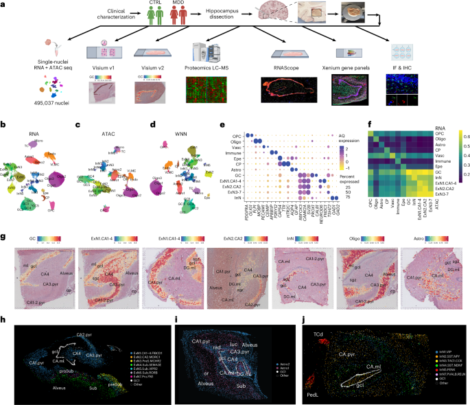
We included 123 participants; 36.45% of samples from the USA and 63.55% from Europe (Extended Data Table 1 and Extended Data Fig. 1a,b). Single-nucleus RNA and ATAC sequencing (snMultiome-seq, 10x Genomics) was performed on hippocampal tissue from 24 CTRL and 12 MDD donors with RNA integrity number (RIN) ≥ 5.7. Following quality control, 74 snMultiome samples (44 CTRL and 30 MDD samples; Supplementary Table 1) from 19 CTRL and 11 MDD donors, with 1–4 technical replicates per donor, were retained for downstream analyses, and Visium v1 and v2 (10x Genomics) were performed on 13 CTRL and 14 MDD donors, each with 1–3 biological replicates (44 samples; Supplementary Table 2). A total of 12 CTRL and 12 MDD samples were used for proteomics, with two biological replicates each. Validation studies included Xenium (four samples), Multiplex RNAscope for PROX1/BHLHE22 + /POSTN (18 samples), Duplex RNAscope for DCX/TUBB3 (22 samples, ACDBio), immunofluorescence for DCX/NeuN (16 samples), immunohistochemistry for nestin (71 samples), Ki67 (42 samples), doublecortin (58 participants), and NeuN (70 samples), and Cresyl Violet staining for Nissl bodies (98 samples).
Tissue processing
The flash-frozen right hemisphere hippocampus was used for all studies. Because we showed fewer GCs selectively in the anterior MDD hippocampus61, the anterior hippocampus proper, including the DG and CA regions, was dissected and sections at 2-mm intervals were used for snMultiome-seq (five 50-μm-thick sections), Visium v1 and v2 (two 16-μm sections), proteomics (two 50-μm sections post-fixed in 4% paraformaldehyde), RNAscope (three 14-μm sections) and Xenium (one 10-μm section). According to the Paxinos Atlas62, the anterior hippocampus coordinates range from MNI −13.99 to −32.37, spanning 13.3–30.8 on the inter-commissural line between the anterior and posterior commissures.
For immunohistochemistry validation studies, serial sections at 2-mm interval throughout the whole rostro-caudal axis of the post-fixed (4% paraformaldehyde) hippocampus (4 cm long in humans), comprising the anterior (anterior to the lateral geniculate), mid (spanning along the extent of the lateral geniculate) and posterior (spanning caudally from the end of the lateral geniculate) portions were used. Post-fixation time as 12 h for every 5-mm of tissue block thickness.
Nissl staining was performed on sections at 1-mm intervals throughout the region used for each experiment for anatomical orientation, and on sections immunolabeled for nestin and NeuN for glia identification, while DCX-immunolabeled sections were counterstained using nuclear red.
Nuclei isolation and library preparation
Tissue (~90 mg) was homogenized with a glass Douce tissue homogenizer (Wheaton, 357542) in 5 ml lysis buffer (10 mM Tris-HCl, pH 7.4, 10 mM NaCl, 3 mM MgCl2 6H2O and 0.05% NP-40), incubated on ice (5 min), quenched in nuclear wash buffer (5 ml, 5% BSA, 0.25% glycerol and 0.001% protector RNase inhibitor in PBS), filtered through a 40-μm Corning cell strainer and centrifuged three times at 500g (5 min, 4 °C). The pellet was resuspended in nuclear wash buffer and the final resuspension was ultracentrifuged at 10,000g (30 min, 4 °C) over an iodixanol cushion (Millipore Sigma, cat. no. D1556-250), adapting a published method63. Nuclei isolation using Singulator (S2 Genomics) was performed by processing tissue (~90 mg) and RNase inhibitor (5 μm) with a nuclei isolation bundle (cat. no. 100-288-798), the lysate was filtered and centrifuged at 500g (5 min, 4 °C), and the pellet was resuspended in 2 ml Nuclei Storage Reagent, centrifuged at 500g (5 min, 4 °C) and resuspended in 3 ml Nuclei Debris Removal Reagent for a final centrifugation at 500g (15 min, 4 °C), obtaining similar yield as with manual extraction. Nuclei concentration (2–9 × 10⁶ nuclei per ml) and viability was estimated using Trypan blue and 4,6-diamidino-2-phenylindole (DAPI) on a Countess II Hemocytometer (Applied Biosystems).
Single-nucleus gene expression (GEX) and ATAC libraries were prepared following Chromium Next GEM Single Cell Multiome ATAC + GEX (CG000338), sequenced on an Illumina NovaSeq 6000 (v4 chemistry, average sequencing depth 83,919 reads/nuclei for GEX and 45,624 for ATAC; Extended Data Fig. 1c–v).
Visium v1 and v2 library preparation
We processed 21 tissue sections with Visium v1 and 23 with v2. The v1 sections were mounted on barcoded slides (6.5 × 6.5-mm capture area), v2 sections on Superfrost slides (11 × 11-mm capture area), stored at −80 °C, fixed, stained and imaged following the 10x User Guide CG000160 Rev C for v1 and CG000164 Rev C for v2. The v2 probes were transferred to the slide using CytAssist. The spatial spot diameter was 55 µm with a 100-µm center-to-center distance between spots for both v1 and v2.
Visium libraries were prepared following the 10x User Guide CG000239 Rev F for v1 and CG000495 Rev G for v2, sequenced on Illumina NovaSeq 6000 (v4 chemistry, sequencing depth 66,512 mean reads per spot for v1 and 78,361 for v2,).
Data were generated using SpaceRanger v.1.3.0 with spatial 3’ v1 chemistry for v1, and v.3.1.2 with spatial probe-based chemistry for v2. The two technologies were analyzed separately.
Proteomics
Shotgun proteomics using liquid chromatography with tandem mass spectrometry (LC–MS/MS), was performed on 48 fixed tissue samples dissolved in 0.2% RapiGest SF in 50 mM ammonium bicarbonate, heated (105 °C for 30 min, then 80 °C for 2 h) and digested with trypsin, run for 120 min, with two chromatograms per biological replicate, using a traveling-wave ion mobility spectrometry MSE mode. Yeast alcohol dehydrogenase (50 fmol) was added as an internal control. Mass spectra were recorded every 0.6 s with a ‘lockmass’ (Glu-1-fibrinopeptide B, m/z 785.8426) recorded every 30 s. Analyzing 792,000 mass spectra, 80,504 peptides and 1,811 proteins were detected at 4% FDR and 1,131 proteins with ≥2 peptides and peptide score >250 were retained for analyses64.
Validation studies
For the Xenium 266-probe and 5050-probe assays, frozen tissue was mounted onto a 10.45 × 22.45-mm sampling area, fixed and permeabilized, and probe hybridization, ligation and amplification were carried out as per 10x Genomics protocols (CG000579, CG000581 and CG000582 Rev C).
Duplex and Multiplex RNAscope were performed on fresh frozen slide-mounted tissue fixed in 4% paraformaldehyde (15 min at room temperature), followed by probe hybridization per ACDBio protocols, including positive and negative control probes. Duplex RNAscope was conducted using a 1:50 ratio of channel 2 (C2, red) DCX probe (cat. no. 489551-C2) to C1 channel (green) TUBB3 probe (cat. no. 601991-C1); the red signal was detected by adding 1:60 Fast Red-B to Fast Red-A, and the green signal was detected by adding 1:50 Fast Green-B to Fast Green-A, slides rinsed and counterstained with 50% hematoxylin (Gil’s Hematoxylin No. 1, Sigma-Aldrich cat. no. GHS132-1L). Multiplex RNAscope was performed following a similar protocol and using probes for POSTN (cat. no. 409181-C1), BHLHE22 (cat. no. 448351-C2), PROX1 (cat. no. 530241-C3) and Multiplex Fluorescent Reagent Kit v2 (cat. no. 323100).
Immunohistochemistry was performed by incubating primary antibodies for 5 days with blocking buffer at 4 °C (anti-nestin mouse monoclonal, 1:8,000 dilution, Chemicon cat. no. ST1111-100UL; anti-Ki67 Novocastra mouse monoclonal 1:1 solution Leica Biosystems cat. no. NCL-L-Ki67-MM1; anti-doublecortin guinea pig polyclonal, 1:30,000 dilution, Sigma-Aldrich cat. no. AB2353; anti-NeuN mouse monoclonal, 1:100,000 dilution, Clone A60, Millipore Sigma cat. no. MAB377) followed by incubation with biotin-conjugated secondary antibodies diluted at 1:200, goat anti-guinea pig (Vector cat. no. PI23227) and horse anti-mouse (Vector cat. no. BA-2000), staining using 0.05% 3,3’-diaminobenzidine or nickel-diaminobenzidine (Millipore Sigma) and counterstaining for Nissl substance with Cresyl Violet16,61.
For immunofluorescence, antibodies (anti-doublecortin guinea pig, 1:1,000 dilution, Millipore cat. no. AB2253; anti-NeuN rabbit monoclonal, Sigma-Aldrich cat. no. MABN140) were incubated in blocking solution overnight at 4 °C, and with secondary antibodies Alexa Fluor 594 goat anti-guinea pig and Alexa Fluor 488 goat anti-rabbit (1:500 dilution, Jackson ImmunoResearch cat. no. 106-585-003 and 111-545-003, respectively) and counterstained with DAPI.
For both immunohistochemistry and immunofluorescence primary antibodies were omitted to exclude unspecific staining16,61.
Cell numbers were estimated in the DG region of interest using unbiased stereology software (Stereo Investigator, MBF)16,61.
Single-nucleus multiome data integration and processing
GEX count matrices and ATAC fragment files were generated using 10x Cell Ranger v.2.0.0 with Single Cell Multiome ATAC + GEX v1 chemistry. Ambient RNA was removed from GEX matrices using SoupX (autoEstCont and adjustCounts, default parameters). Cells were retained if they contained 500–150,000 UMIs, >300 genes and <10% mitochondrial RNA, consistent with published filtering strategies for high-sensitivity 10x datasets63 and rare neurogenic cell populations3. Low-quality cells (<300 genes and >10% mitochondrial RNA; Supplementary Fig. 1a) and doublets identified using scDblFinder were removed.
ATAC peak BED files were converted to GenomicRanges objects and merged into a unified peak set. Peaks on nonstandard chromosomes, within hg38 blacklist regions, or >10 kb or <20 bp were removed. Cells with transcription start site enrichment <1, nucleosome signal >3 or 200–100,000 ATAC reads were excluded (Supplementary Fig. 1a).
All 74 samples were merged in both modalities. Cells that passed quality control were retained for further analysis.
GEX data were processed with Seurat. After normalization (NormalizeData), the top 2,000 highly variable genes were identified (FindVariableFeatures) and, together with 93 curated neurogenesis-associated genes, scaled using ScaleData. Principal-component analysis (PCA) (RunPCA) was performed, and the top 40 principal components (PCs) were batch-corrected with Harmony (RunHarmony) using sample, donor and batch as covariates (Supplementary Fig. 1b–e).
ATAC data were processed with BPCells and Signac. BPCells enabled disk-backed storage of the peak matrix. Peaks were TF-IDF normalized, reduced by latent semantic indexing (LSI), and batch-corrected with Harmony using LSI components 2–40 and donor, sample and batch as covariates (Supplementary Fig. 1f,g).
WNN analysis was performed with FindMultiModalNeighbors using the top 30 Harmony-corrected PCs and LSI embeddings (prune.SNN = 1/20). The resulting graphs were used for UMAP and Leiden clustering (FindClusters, algorithm = 4, resolution = 0.8).
Differential gene expression across the 31 clusters was assessed by pseudobulk linear mixed-effects modeling with SpatialLIBD, including sample, batch, sex, scaled age and winsorized RIN and post-mortem interval (PMI, time from demise to brain collection, measured in hours) as fixed effects and donor as a random effect. Clusters were annotated using canonical gene expression per human hippocampus snRNA-seq studies3,4,36,65,66 (Fig. 1e and Extended Data Fig. 2a).
Data were integrated with published snRNA-seq datasets3,36,65,66 (Extended Data Table 2) using reciprocal PCA integration. External datasets were preprocessed with Seurat67 and Harmony, and cluster correspondence was assessed by Pearson correlation of average expression across the top 5,000 variable genes (Extended Data Fig. 3a–m).
Multiome neurogenic cell trajectory identification
Because one astrocyte cluster (Astro2) and one GC cluster (GC2) expressed immaturity-associated genes3,36,65,66, we hypothesized that GC and astrocyte populations contained neurogenic cells. We therefore subset these clusters and repeated the Seurat workflow (normalization, dimensionality reduction, Harmony integration, WNN analysis and clustering), identifying 17 unsupervised clusters. Among the 17 clusters obtained, we selected cells enriched with known early, intermediate and late neurogenesis markers3,4,36, and then applied FindSubClusters at 0.5 resolution.
We annotated cell clusters based on their enrichment with canonical neurodevelopmental and neurogenesis-associated markers and, for visualization purposes, the remaining mature GC and astrocyte clusters were merged together as mGC and mAstro, whereas GC4 was maintained separately as it expressed immune and GC markers, suggesting microglia engulfment (Fig. 2a,b). Cells were annotated as NSCa when expressing neuronal-lineage-associated ASCL1 with SOX2 (ref. 16), RMST, a long noncoding RNA regulating neurogenesis by interacting with SOX2 (ref. 16), PAX6 (ref. 68) and LAMA2 (ref. 69), encoding an ECM protein that maintains NSC niches, promotes progenitor survival and dictates the transition from stem cells, and RSPO2, essential for neurogenesis. Cell defined as NSCb expressed NES16, FABP5 and FABP7, regulators of NSC proliferation and survival, ID3 (ref. 70), which inhibits early differentiation, SFRP2, a modulator of the Wnt signaling pathway and TPPP3, encoding a microtubule-associated protein that regulates microtubule dynamics, bundling, and cell mitosis. Cells were annotated as INPs when enriched with neurogenic STMN1 and STMN2 (ref. 18), TUBB3 (ref. 17), NNAT3,4 and NEUROD6. NBs were identified by expression of classic neurogenic marker DCX16, with ST8SIA2 (ref. 16), which drives polysialylation, CALB2 (refs. 3,4), RELN15 and NELL1 found in neuroblasts and neuroblastoma cells. Two clusters expressing PROX1 were annotated as immature GCs: ImGC1, expressing INSM1, encoding for zinc-finger TF involved in embryonic neurogenesis, and NEUROD1 (refs. 3,4), necessary for neuronal differentiation, whereas ImGC2 expressed developmental genes BHLHE22 (ref. 6), FST9, OTOF71, POSTN7 and SMAD7 (ref. 24).
Clusters were validated by applying gene signature scoring with ScoreSignatures_UCell using canonical markers for NSCs, INPs, NBs and ImGCs3,4,18 as features (Fig. 2c).
To compare transcriptional profiles of the putative adult neurogenic trajectory with embryonic neurogenic cells, we integrated NSCa, NSCb, INP, NB, ImGC1 and ImGC2 data with a fetal hippocampus snRNA-seq dataset68 (in Seurat using reciprocal principal component analysis (PCA) with SCTransform (SCT) normalization and 3,000 integration features), including fetal PROX1+ GCs, AQP4+ astrocytes and three types of ASCL1+ progenitors, while OPCs were excluded (Extended Data Fig. 4b–d).
Neurogenic cell trajectory inference
Neurogenic trajectories were inferred with Monocle72 and Palantir73, using NSCa as the root population. Pseudotime, terminal state probabilities and entropy were computed, and gene expression was denoised with MAGIC. Gene expression dynamics and modules were analyzed, and the neurogenic subtrajectory was isolated for downstream analyses. For visualization and analysis, neurogenic populations were randomly downsampled to 10,000 cells each. Trajectory-dependent differential gene expression was assessed with Monocle3 using the model pseudotime × diagnosis.
Transcription factor binding analysis on cell trajectory clusters
TF regulation along the neurogenic trajectory was analyzed using TOBIAS74 and pySCENIC (Fig. 2h). Neurogenic ATAC peaks were called with Signac75 CallPeaks from MACS3, corrected for Tn5 bias, footprinted and analyzed with BINDetect to infer TF-binding dynamics using JASPAR76 motifs, excluding ENCODE blacklist regions. Peaks were annotated with UROPA, and TF activity visualized using motif binding z-scores. Gene regulatory networks were inferred from GEX data with PySCENIC72 (GRNBoost2; Fig. 2i), pruned, and repeated 50 times to retain robust regulons (>20% of runs; Fig. 2i). AUCell scores were calculated for each cluster, and regulon activity was compared to TF-binding dynamics to identify stage-specific regulatory programs.
Spatial gene expression data processing, integration and cluster annotation
Visium v1 and v2 data were loaded into Seurat (Load10X_Spatial), normalized, variable features identified and data scaled using standard Seurat workflows. Replicates were merged and PCA, UMAP, neighbor graph construction and clustering were performed using the top 30 PCs; spots with fewer than 500 UMIs were excluded from downstream analyses.
Unsupervised spatial clusters were identified with Seurat (FindClusters, resolution of 0.34) and annotated by marker gene expression and hippocampal anatomy. Low-abundance clusters were removed, yielding 13 clusters in Visium v1 and 17 in Visium v2 (Extended Data Fig. 4e,f and Supplementary Figs. 2 and 3), each represented across all samples. Shared clusters included the granule cell layer, SGZ (with molecular and polymorphic layers), choroid plexus, inhibitory neurons, axons, dendrites and vasculature. Visium v1 contained a combined stratum lucidum/radiatum cluster, whereas v2 resolved these into separate lucidum and radiatum clusters and identified a distinct CA2 cluster.
Differential gene enrichment analysis was performed on each cluster by pseudobulked linear mixed-effects modeling, including sample, batch, sex, scaled age and winsorized RIN and PMI as fixed effects, and donor as a random effect, implementing the SpatialLIBD package77.
Integration of single-nucleus and spatial transcriptomic data
To determine how snMultiome-seq cell clusters anatomically map onto hippocampus subfields, anchor-based integration using snMultiome-seq as reference and Visium v1 and v2 and Xenium as query datasets was performed by FindTransferAnchors and TransferData in Seurat67, assigning spatial spots probability scores based on transcriptional congruence (Fig. 1g–j).
Neurogenic niche spatial trajectory inference by RNA velocity on Visium data
To probe the existence of a trajectory in the DG neurogenic niche, gene expression dynamics across hippocampus spatial clusters were analyzed, focusing on sgz.pl, sgz.ml and gcl, which expressed proliferation, differentiation, maturation and neurogenesis markers among their top 100 (Extended Data Fig. 4e,f).
RNA velocity was computed on Visium v1 (55 × 55μm spots, poly(A)-based) using velocyto78 and scVelo following BAM sorting with SAMtools. Velocity was estimated using the dynamical model after PCA on the top 5,000 variable genes plus 55 neurogenesis-associated genes and construction of a 30-nearest-neighbor graph, PAGA was used to infer connectivity and branching between spatial spots, and latent time to estimate where each spots lay between the beginning and end of a trajectory (Extended Data Fig. 4g,h).
Statistical analyses comparing participant and biospecimens characteristics
Pairwise comparisons were performed using two-sided Wilcoxon rank-sum tests for age, PMI, brain pH, RIN and snMultiome RNA/ATAC quality metrics and chi-squared tests were used to compare sex distribution between MDD (n = 55) and CTRL (n = 68) participants (Extended Data Fig. 1c–l). Resulting P values were adjusted for multiple comparisons using the Benjamini–Hochberg FDR procedure and an FDR-adjusted P value < 0.05 was considered statistically significant.
Linear regression analyses were performed within diagnostic groups to assess relationships between RIN and age, PMI and brain pH in the full cohort with available RIN values (n = 76 participants), and in cohort selected for the omics studies (n = 38 participants and 74 samples; after removing 3 samples after quality control; Extended Data Fig. 1m–v and Supplementary Table 1) with a P value < 0.05 considered as statistically significant.
Analysis of differential gene expression and accessible chromatin in MDD versus CTRL
Differential gene expression and chromatin accessibility between MDD and CTRL were analyzed on cluster-level pseudobulk data using limma. Count and peak matrices were aggregated by biological sample and cluster without merging samples from the same donor processed in different batches. Pseudobulks with fewer than five cells or spots were excluded. Models included cell/spot number, winsorized RIN and PMI, age, sex, sample and batch as fixed effects, with within-donor correlation estimated using duplicateCorrelation. Lowly expressed genes were filtered with filterByExpr (edgeR), normalized using TMM (calcNormFactors), and analyzed with voomWithQualityWeights, lmFit and eBayes to account for variable sample quality and repeated donor measurements. For NSCs, INPs and NBs, DEG significance was defined as P < 0.05 log2FC > 1 to reduce type II error due to low cell numbers (Fig. 3h); for visualization only, these findings were shown in a single volcano plot. For ImGC1, ImGC2 (Fig. 3i), all other snMultiome clusters (Fig. 4a), and all Visium v1/v2 clusters (Extended Data Fig. 7a,b), DEGs were defined as FDR < 0.05 and log2FC ≥ 0.5.
Differential protein expression analysis between MDD and CTRL
Proteomic data were analyzed with the Rosetta Elucidator Protein Expression Analysis System, and peptide identifications were assigned with Mascot against the UniProt/SwissProt human canonical protein database with isoforms. DEPs were defined as those with >2 peptides and P < 0.05. Duplicate protein accessions were collapsed before Reactome pathway enrichment using ReactomePA and clusterProfiler (Benjamini–Hochberg correction; minGSSize = 10, maxGSSize = 500), and related pathways were grouped into parent categories (Fig. 5a,b).
Differential transcription factor binding analysis in MDD versus CTRL
Following differential chromatin accessibility analysis, TF-binding activity between MDD and CTRL was inferred across all snMultiome cell clusters using TOBIAS74 (Fig. 6b). Cluster-specific peaks were called with MACS375 via Signac75, corrected for Tn5 bias (ATACorrect), footprinted (ScoreBigWig), and analyzed with BINDetect to identify differential TF binding between MDD and CTRL (Fig. 6d,f,h). ENCODE blacklist regions were excluded, peaks were annotated with UROPA, and vertebrate TF motifs were obtained from JASPAR76. BINDetect results were filtered to TF motifs with differential binding (P ≤ 0.01) and only predicted target DEGs retained in the corresponding cluster and overlapped with DEPs (Fig. 6c,e,g). These TF–target pairs were used to construct regulatory networks linking TF binding, gene expression and protein expression, with edge weights representing log2 differential binding scores and gene nodes colored by DEG logFC (Fig. 6c,e,g). KLF15 binding profiles at target loci were visualized using PyBigWig and Matplotlib (Fig. 6d,f,h).
Cell abundance estimation in MDD versus CTRL
Differences in neurogenic cell proportions between MDD and CTRL were tested using β-binomial generalized linear mixed models (glmmTMB) in each neurogenic cluster using the same covariates as for the differential gene expression and accessible chromatin analyses (Fig. 3c).
Duplex RNAscope, immunohistochemistry and immunofluorescence data were compared between MDD and controls using Welch’s t-test in Prism (Extended Data Fig. 6d,e).
For Multiplex RNAscope, linear models in R (using the same covariates as for the differential gene expression and accessible chromatin analyses) tested the effect of MDD on the abundance of GCL and SGZ cells coexpressing PROX1 with POSTN or BHLHE22, or all three markers (Extended Data Fig. 6g,h).
High-dimensional weighted gene coexpression network analysis
The hdWGCNA79 was performed in Seurat67 on all unsupervised clusters (Fig. 4e–g). After normalization, scaling and Harmony batch correction, metacells were generated within each cluster-sample group (≥100 cells; 20 Harmony dimensions, k = 25). Signed coexpression networks were constructed, gene modules were identified and module eigengene connectivity (kME) was calculated. Reactome pathway enrichment was assessed using Enrichr via the hdWGCNA pipeline. Module–diagnosis associations were tested with linear mixed-effects models, including diagnosis as a fixed effect, sample and batch as random effects, and age, PMI and RIN as covariates, with Benjamini–Hochberg FDR correction.
Pre-ranked gene set enrichment analysis
Pre-ranked GSEA was performed with clusterProfiler using genes ranked by logFC × −log10 (Benjamini–Hochberg-adjusted P value). Differentially regulated KEGG and Reactome pathways were identified (minGSSize = 10, maxGSSize = 400, P < 0.05, including Benjamini–Hochberg FDR correction) and related pathways were collapsed into parent categories.
Analysis of trans-diagnostical involvement of MDD dysregulated genes and proteins
Neuropsychiatric disease enrichment was assessed using psygenet2r (PsyGeNET80; database = ‘ALL’). Cell cluster significant DEGs (Extended Data Fig. 7c,d) and DEPs (Fig. 6f,g) were analyzed with psygenetGene to identify associated psychiatric disorders.
Reporting summary
Further information on research design is available in the Nature Portfolio Reporting Summary linked to this article.