
The research in this study complies with all relevant ethical regulations. The protocols used to generate our snRNA-seq and bulk RNA-seq data were approved by the institutional review board of the Dana-Farber/Harvard Cancer Center. Protocols related to the NHS/HPFS validation cohort were approved by the institutional review boards of Brigham and Women’s Hospital and the Harvard T.H. Chan School of Public Health. Written informed consent was obtained from all participants, who were not compensated. For the snRNA-seq and bulk RNA-seq cohorts, the obtained consent allows samples and clinical information to be shared with internal and external collaborators for gastrointestinal cancer research. Patient sex was collected from clinical records. As all available tissue was processed, sex was not considered in the study design. Sex, age and other clinical metadata are reported in a disaggregated manner in Supplementary Table 1 (snRNA-seq) and Supplementary Table 4 (bulk RNA-seq). The ages of patients 90 years and older have been aggregated into a single ‘90+’ category. For the NHS/HPFS multispectral immunofluorescence cohort, sex was self-reported and was only considered in the study design due to the nature of the cohort compositions (NHS is a cohort of women and HPFS is a cohort of men). Aggregated clinical metadata are reported in Supplementary Table 5. Instructions for accessing the aggregated clinical metadata are provided in the Data Availability statement.
Patient samples and clinical data
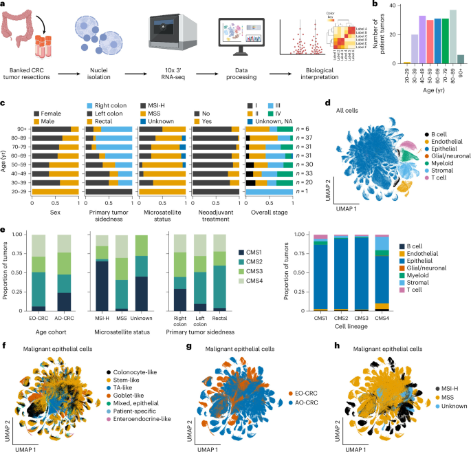
Primary colorectal tumor samples with a pathologic diagnosis of adenocarcinoma were collected from the operating room from patients who consented to participate in research under Dana-Farber/Harvard Cancer Center Protocols 03-189, 11-104, 14-091, 14-408, 17-000 and/or 20-000. Tumors were snap-frozen and stored at −80 °C in the DFCI Gastrointestinal Cancer Center Biobank. Demographic, clinical, pathologic and molecular characteristics, as well as treatment data, were manually abstracted from the medical records by a team of clinical research coordinators from the DFCI Gastrointestinal Cancer Center Biobank. The final cohort included 189 primary tumor samples collected from 189 unique patients.
Cohort statistical associations and enrichments
Associations between age cohort and clinical metadata were evaluated using chi-square tests (chi2_contingency) from SciPy (v1.14.1), and P values were adjusted for multiple comparisons using the multipletests function in statsmodels (v0.14.2) to calculate the Benjamini–Hochberg FDR. Patients with missing values for the association being tested were excluded from the analysis. To calculate enrichment within an age cohort of a specific metadata category, ORs with 95% CIs and associated P values were computed using Fisher’s exact test (fisher_exact) and the Table2x2 class from statsmodels.
Nuclei isolation, library construction and sequencing
A biopsy-sized (∼3 mm2) piece of tissue was manually chopped in CST dissociation buffer for 10 min on ice20. The dissociated tissue was then filtered through a 40-μm strainer (pluriSelect, 43-10040-60) and centrifuged at 500g and 4 °C for 10 min. The nuclei were resuspended in PBS (Gibco, 10010031) with 1% BSA (Miltenyi Biotec, 130-091-376), filtered and counted after staining with 4′,6-diamidino-2-phenylindole (DAPI) (Sigma-Aldrich, D9542-1MG). Approximately 12,000 nuclei were loaded onto a 10x Chromium Controller and processed using the 10x 3′ v3.1 dual index assay (10x Genomics, 1000268). Following single-nuclei barcoding, reverse transcription and library construction were performed according to the manufacturer’s guidelines (10x Genomics). Samples were sequenced on a NovaSeq 6000 using S2 flow cells (Illumina) with the following dual-indexed, paired-end read configuration: read 1, 28 nucleotides (nt); read 2, 90 nt; index read 1, 10 nt; index read 2, 10 nt.
Data preprocessing, quality control and atlas integration
Raw sequencing files were demultiplexed using bclconvert (v3.10.5)71, run with the Terra Workflow Description Language (WDL). Gene expression count matrix was generated using Cell Ranger v7.0.1 (through the Cumulus v2.3.0 WDL72,73 on Terra74). Ambient RNA counts and empty droplets were removed using CellBender remove-background (v0.2.0)75,76. The Cumulus WDL was used to further remove nuclei with fewer than 200 genes, fewer than 400 UMIs or more than 50% of counts mapped to mitochondrial genes72,77. Count matrices from individual samples were integrated using Scanpy (v1.10.2), after which Cumulus-predicted doublets were removed, as well as cells with ≥10,000 genes or ≥50,000 UMIs. Cells in the integrated atlas were normalized to 1 × 10⁴ total UMIs and log-transformed. Highly variable genes were selected using scanpy.pp.highly_variable_genes (min_mean = 0.0125, max_mean = 3, min_disp = 0.5) from Scanpy. Principal component analysis (PCA) was performed using scanpy.tl.pca (svd_solver = ‘arpack’); nearest neighbors were calculated using scanpy.pp.neighbors (n_neighbors = 10, n_pcs = 40); a UMAP embedding was generated using scanpy.tl.umap; and Leiden clustering was performed using scanpy.tl.leiden—all implemented in the Scanpy package.
Cell subset annotation
Cells were annotated at both the lineage and granular levels. Seven lineage-level annotations (epithelial, myeloid, B, T, endothelial, glial/neuronal, stromal) were assigned to each Leiden cluster (resolution = 0.1) using published27 gene signatures for colon cells. Selected marker genes for each lineage are shown in Extended Data Fig. 2b. Granular annotations were assigned by subclustering raw counts within each lineage, followed by normalization, log transformation, calculation of variable genes and PCA, as described above. Within each lineage except glial/neuronal, we then performed patient batch correction using scanpy.pp.harmony_integrate from harmonypy (v0.0.10)78, generated a UMAP and performed Leiden clustering at multiple resolutions. For the glial/neuronal subset, UMAP, clustering and annotation were performed without batch correction due to the smaller number of tumors. Non-batch-corrected UMAPs for all lineage subsets were also generated to facilitate the visualization of annotations and clinical metadata.
Clusters were annotated using a mix of published gene signatures26,27, canonical cell type markers, calculated marker genes and celltypist.annotate from CellTypist (v1.6.3)79,80 (model = Cells_Intestinal_Tract, model = Human_Colorectal_Cancer). Gene signatures were scored using scanpy.tl.score_genes, and marker genes were identified using scanpy.tl.rank_genes_groups from Scanpy (v1.10.2). The top 30 marker genes for the selected granular epithelial subsets are shown in Extended Data Fig. 3b. These subset markers, as well as the marker genes for the Leiden clusters from each lineage subset, are provided in Supplementary Table 2. In the epithelial subsets, three small patient-specific clusters remained after batch correction. Two of these clusters (6 and 7) were merged with the closest major epithelial subset based on transcriptional similarity; the third cluster was sufficiently distinct to be annotated as a separate patient-specific cluster.
CMS and iCMS classification
The CMS for each sample was classified using CMScaller22,23 (v2.0.1) in R. Raw counts for all cells in the atlas were pseudobulked per tumor using the get_pseudobulk function (mode = ‘sum’, min_cells = 10, min_counts = 1000) from the decoupleR package (v1.8.0) in Python. Genes expressed in at least 10% of samples in either the AO-CRC or EO-CRC cohort were retained using filter_by_expr (min_prop = 0.1, min_count = 10) from decoupleR. Gene symbols were converted to Ensembl IDs using getBM from the biomaRt package (v2.58.2) in R, and pseudobulk counts for each sample were classified using CMScaller with the single-sample prediction (SSP) protocol. A two-sided Fisher’s exact test was used to determine the enrichment of each CMS with age (one versus all). Associations between specific CMSs (one versus all) and age were further evaluated using the logit function from the statsmodels package (v0.14.6) in Python to run a logistic regression analysis modeling age scaled to unit variance (z-scored) as a continuous variable with microsatellite status, sidedness, neoadjuvant treatment history, sex and stage as covariates. Significance was determined using a two-sided Wald test. Rectal and treated samples were removed from the CMS1 multivariable logistic regression test because no samples in these clinical groups were classified as CMS1.
iCMS2/3 scores were calculated using scanpy.tl.score_genes from Scanpy (v1.10.2) and the published gene sets from Joanito et al.43. To determine associations between mean iCMS2/3 scores and age as well as other clinical covariates, a multivariable linear regression was fit using ordinary least squares (OLS) in the statsmodels package (v0.14.6) in Python, modeling age scaled to unit variance (z-scored) as a continuous variable with microsatellite status, sidedness, neoadjuvant treatment history, sex and stage included as covariates. Tumors with unknown clinical metadata for any included covariate were excluded from the analysis. Significance was determined using a two-sided t test.
Compositional changes and principal coordinates analysis
Changes in cell subset composition across the age continuum were identified separately in the MSS and MSI cohorts using the DirichReg R package (v0.7.1), with age scaled to unit variance (z-scored) as a continuous variable and sidedness, neoadjuvant treatment history, sex and stage as covariates. At the lineage level, we ran Dirichlet regression in two ways: (1) using the ‘common’ model with no reference variable, where all cell types are modeled relative to each other and (2) using the ‘alternative’ model with epithelial cells as the reference variable. For the common model, we used counts ~ age_scaled + sideness + therapy + sex + stage as the design formula; for the alternative model, we used counts ~ age_scaled + side + therapy + sex + stage | age + side + therapy + sex + stage. Multiple hypothesis correction was performed across P values for all covariates by calculating the Benjamini–Hochberg FDR using p.adjust(pvals, method = ‘fdr’) in R. Dirichlet regression (common model and design formula indicated above) was also performed using all granular cell types. For the MSS tumors only, we further evaluated compositional changes in the granular subsets within the epithelial compartment (common model). Lineage-level compositional changes were confirmed using scCODA integrated into the pertpy package (v1.0.5) in Python, by applying the prepare, run_nuts and get_effect_df functions with default hyperparameters. In the scCODA analysis, each cell type was iteratively set as the reference cell type; min–max normalized age was modeled continuously with sidedness, neoadjuvant treatment history, sex and stage as covariates; and the final parameters were evaluated (posterior inclusion probability > 0.95 in all iterations). Principal coordinates of cell type composition were calculated from Bray–Curtis dissimilarities of lineage-level cell type proportions per sample, using the pco function from the labdsv R package (v2.1.0). Granular annotations with ‘mixed-marker’ assignments (that is, a mix of markers from the assigned lineage as well as other lineages) were excluded from all composition analyses27.
inferCNV
CNAs were inferred using inferCNV (v1.19.1)38, run with the Terra WDL infercnv_wf81. The WDL was run once per tumor sample, with epithelial cells as the test group and all nonepithelial cells as the reference. Cell subset annotations that showed marker gene expression from multiple lineages (containing ‘mixed’ in their name) were excluded from the analysis. The following arguments were specified: –analysis_mode = ‘subclusters’ –HMM –denoise –cutoff = 0.1 –leiden_function = ‘modularity’. Two samples (COLFR0034_T1, COLFR0366_T1) were excluded from the downstream analysis because they had insufficient counts within one or more subsets.
The heatmaps in Fig. 3a and Extended Data Fig. 5a,c were generated by extracting the HMM cell state information from HMM_CNV_predictions.HMMi6.leiden.hmm_mode-subclusters.Pnorm_0.5.pred_cnv_genes.dat, resulting in a matrix of CNA subclusters by genes, with entries ranging from 1 to 6 (values of 1 and 2 indicate deletions; 3 indicates no CNA; 4–6 indicate duplications). Genes without a predicted cell state were assigned a default value of 3, and the genes were ordered according to their locus. The resulting cell states were clustered using the clustermap function from the Seaborn Python package (v0.13.2), with row distances calculated using pdist and linkage from SciPy (v1.14.1; method = ‘ward’ and metric = ‘correlation’). Clustering was performed separately for the MSS and MSI samples in our cohort.
To assess the consistency of the predicted CNAs with known losses and gains in bulk RNA-seq cohorts, reference CNA profiles were accessed from cBioPortal on June 10, 2026; only samples with a MANTIS score of <0.4 (MSS) were used for comparison. For comparison to CNAs in adjacent normal tissue from the Pelka et al.26 cohort, we ran inferCNV as described above on MSS tumor samples and the adjacent normal samples. The CNA subclusters from the Pelka et al.26 samples were then clustered with the CNA subclusters from the MSS samples in our atlas. To evaluate age associations among the three CNA metaclusters formed across the MSS tumor samples in our cohort, we separately compared the high CNA and moderately high CNA metaclusters to the low CNA metacluster using a multivariable mixed-effects regression model with patient ID (that is, tumor sample) as a random effect, as there can be more than one CNA subset per tumor. We performed this analysis in R using glmer from the lme4 package (v1.1.38), again using age scaled to unit variance (z-scored) as a continuous variable: cluster ~ age_scaled + side + treat + stage + sex + (1 | patient_id) and family = binomial. Significance was determined using a two-sided Wald test.
CNA burden was calculated per cell by summing the absolute values of the log2-transformed CNA residual expression from the object: run.final.infercnv_obj. To evaluate the overall CNA burden per tumor across the age continuum, we averaged the per-cell absolute log2 values within each tumor and performed multivariable linear regression using OLS implemented in the statsmodels package (v0.14.6) in Python, modeling scaled age as a continuous variable with sidedness, neoadjuvant treatment history, sex and stage as covariates. Significance was determined using a two-sided t test.
To assess the change in the likelihood of having two or more and three or more CNA subsets per tumor with age, we used a multivariable logistic regression method (logit from statsmodels), again modeling scaled age continuously with sidedness, neoadjuvant treatment history, sex and stage as covariates. In this regression, we also added a covariate for the mean UMI count per tumor as a proxy for sequencing depth and a covariate for the total number of epithelial cells to capture bias due to detection power. Significance was determined using a two-sided Wald test.
Common gene programs using cNMF
To identify recurrent, shared malignant epithelial gene programs separately within the EO-CRC and AO-CRC cohorts, we used a two-stage workflow adapted from Kinker et al.46, which first identified gene programs specific to individual tumors and then metagene programs at the age cohort level.
Patient-specific gene programs
We first ran cNMF44 separately on the raw counts from the epithelial cells of each MSS left-sided tumor sample. Samples with fewer than 100 epithelial cells were excluded, and genes were filtered to retain protein-coding genes expressed in three or more cells (n = 24 EO-CRC and 25 AO-CRC tumor samples). We used the cNMF package (v1.6.0) in Python and tested a number of factorization ranks (k = 4–15). Each cNMF run was performed on the variable genes, calculated from normalized and log-transformed counts using scanpy.pp.highly_variable_genes (min_mean = 0.0125, max_mean = 5, min_disp = 0.5, flavor = ‘seurat’) from Scanpy (v1.10.2), with 100 iterations, random_seed = 14 and parallelization across four workers.
We ultimately selected k = 10 for each tumor based on visualization of the stability and error metrics from the k_selection_plot function, displayed across all tumors (Extended Data Fig. 6a). We also visualized the program usage scores on individual tumor UMAPs at various values of k to assess the activity of each program (see Extended Data Fig. 6b for a summarized visualization of this process). Our final selection of k = 10 provided a balance of stability and interpretability across tumors from each age cohort. Consensus gene programs were computed using the consensus command from cNMF for the selected k and a density threshold of 0.2.
Within each tumor sample, the cNMF usage values were normalized to sum to one within each cell and stored as observation-level metadata in each tumor’s AnnData object. Additionally, cNMF z-scores for each gene were added to the AnnData object for each tumor as gene-level metadata, representing gene-level contribution weights to each tumor-specific gene expression program (GEP). Separately within the EO-CRC and AO-CRC age cohorts, the top 50 genes were identified for each tumor-specific GEP z-score across all tumors in the age cohort based on sorted z-scores.
Age cohort metagene programs
GEP scores for each tumor-specific program were calculated across all cells in each age cohort using the scanpy.tl.score_genes function in Scanpy (v1.10.2). The mean tumor-specific program scores were visualized using the clustermap function from the Seaborn Python package (v0.13.2). The rows and columns were clustered using the pdist and linkage functions from SciPy (v1.14.1; method = ‘ward’ and metric = ‘correlation’), with rows representing the tumor-specific gene programs (10 programs × 24 tumors = 240 programs in EO-CRC and 10 programs × 25 tumors = 250 programs in AO-CRC) and columns representing the individual samples.
Metagene programs that were active across the EO-CRC and AO-CRC tumor cohorts were identified using unsupervised row clustering. These metaclusters represent robust and recurrent gene programs within each age cohort. We chose the final number of metaclusters per cohort using four criteria: (1) visualization of the resulting metaprograms on individual tumor UMAPs; (2) the overall activity level and patient specificity of the resulting metaprograms scored across all cells within an age cohort; (3) visualization of the mean program scores on the heatmap; and (4) the mean silhouette score. We ultimately selected five metaclusters per age cohort because this provided the best balance among the four metrics mentioned above. The top 50 genes for each EO-CRC and AO-CRC common gene program were determined by sorting the mean z-scores from the common gene program cluster tumor-specific GEPs.
Metagene program evaluation
Similarity between age cohort-specific gene programs was determined by calculating the Jaccard distance between all pairs of EO-CRC and AO-CRC programs. To determine gene program alignment with epithelial granular subsets, the top 50 genes for common programs within each age cohort were scored using scanpy.tl.score_genes, and the scores for each program were visualized with violin plots grouped by cell subset. Enriched pathways were calculated for the top 50 genes within each EO-CRC and AO-CRC cNMF common (as well as age cohort-specific) gene program. Enrichment was performed using the enricher function from the clusterProfiler package (v4.10.1; pAdjustMethod = ‘BH’), using collections from MSigDB (msigdbr v25.1.0) and the default background (all genes appearing in the MSigDB collection). Significance was determined using a one-sided Fisher’s exact test.
Differential gene expression
Within each granular subset, single-cell data were pseudobulked by summing raw UMI counts across cells separately for each tumor, using the get_pseudobulk function (mode = ‘sum’, min_cells = 10, min_counts = 1000) from the decoupleR package (v1.8.0) in Python. Genes were filtered to require expression in at least 10% of samples in either the AO-CRC or EO-CRC cohort using filter_by_expr (min_prop = 0.1, min_count = 10).
Differential expression was tested for the MSS tumors within each granular subset using the pseudobulked data. This analysis was performed using the DESeq2 package (v1.42.1) in R, with age scaled to unit variance (z-scored) modeled continuously and sidedness, neoadjuvant treatment history, sex and stage included as covariates (~sidedness + neoadjuvant_treatment + sex + stage + age_scaled). We applied an additional MSS-specific filter so that only genes expressed in at least 1% of EO-CRC or AO-CRC cells within a granular subset, as calculated at the single-cell level using the Seurat v5.1.0 framework in R, were tested for differential expression. Differential expression was not calculated for granular annotation subsets with fewer than three EO-CRC or AO-CRC samples. If there were fewer than three samples in a given covariate category (across both age cohorts) within a granular subset, that covariate was dropped from the design formula. All tested malignant epithelial subsets had sufficient samples to include all covariates.
Genes with FDR < 0.05 were considered differentially expressed, with a negative log2(FC) indicating decreased expression with increasing age (that is, highest expression in EO-CRC) and a positive log2(FC) indicating increased expression with increasing age (that is, highest expression in AO-CRC). DEGs along the age continuum were visualized using EnhancedVolcano (v1.20.0).
lncRNA enrichment
We annotated genes in our atlas as lncRNAs using the useEnsembl function from the biomaRt package (v2.58.2) in R. Additionally, we included uncharacterized genes beginning with A and ending with a decimal point in our set of lncRNAs. To determine the enrichment of lncRNA genes within DEG sets from each granular subcluster, we performed a two-sided Fisher’s exact test (fisher.test) using the stats package (v4.3.3). P values from granular subsets with more than zero DEGs were adjusted for multiple comparisons using p.adjust (method = ‘fdr’).
GTEx aging signatures
The GTEx82 aging signatures for the sigmoid and transverse colon were downloaded from the repository70 at https://doi.org/10.5281/zenodo.6797627 and filtered for genes with an adjusted P value of <0.05. Genes with positive and negative FC values were labeled as having increased and decreased expression with age, respectively. These genes were intersected with DEGs and gene program lists from our snRNA-seq analyses to ensure that the identified genes were not primarily driven by patient age. DEGs along the age continuum from the GTEx cohort were visualized using EnhancedVolcano (v1.20.0).
Cell–cell interaction
CellChat 2.0 (v2.1.2) was run separately for the EO-CRC (n = 25 tumor samples) and AO-CRC (n = 26 tumor samples) MSS left-sided tumor cohorts to identify cell–cell interactions. Before running CellChat, cells belonging to granular subsets with ‘mixed’ annotations were removed. The CellChat analysis was performed at an intermediate annotation level, including granular epithelial cell annotations to facilitate subset-specific analysis and lineage-level annotations for the nonepithelial cells to maximize power. Raw counts were scaled (1 × 10⁴) and log-normalized using NormalizeData from Seurat (v5.1.0). These normalized counts were used to create an age cohort-specific MSS left-sided CellChat object through createCellChat, grouped by the intermediate annotation level with datatype = ‘RNA’.
CellChatDB.human was used as the interaction database, including only interactions annotated in the CellChat database and excluding non-protein signaling interactions. Genes were subsetted to those present in the database, and overexpressed genes and interactions were identified. Communication probability between intermediate-level cell types was calculated using computeCommunProb, with the triMean method and nboot = 1000. Interactions involving fewer than ten cells were filtered using filterCommunication; communication probabilities were aggregated at the pathway level using computeCommunProbPathway; and a communication network was built using aggregateNet.
After identifying the cell–cell interactions separately for the EO-CRC and AO-CRC MSS left-sided tumor samples, the number of interactions for each age cohort was compared using compareInteractions (overall) and netVisual_heatmap (grouped by cell type and split by sender or receiver role). Differences in interaction strength at the pathway level were assessed using rankNet (mode = ‘comparison’, measure = ‘weight’, do.stat = TRUE); this function identifies pathways that are significantly different between the age cohorts using a two-sided Wilcoxon (Mann–Whitney U) test with a P-value cutoff of 0.05. Interaction differences between cell types at the pathway level were visualized using netVisual_aggregate.
Bulk RNA-seq validation data
TCGA-COAD and TCGA-READ bulk RNA-seq data
Clinical and RNA-seq data were obtained for the COAD-US and READ-US projects of TCGA on March 5, 2026. TCGAbiolinks (v2.37.1) was used in R (v3.4.0) to query the NCI Genomic Data Commons (GDC) portal as follows: project = c(‘TCGA-COAD’, ‘TCGA-READ’), data.category = ‘Transcriptome Profiling’, data.type = ‘Gene Expression Quantification’, experimental.strategy = ‘RNA-Seq’, workflow.type = ‘STAR – Counts’ and access = ‘open’.
MSI status was obtained directly from the GDC portal’s ‘MSI status’ filter in the Repository tab and mapped to TCGA-COAD and TCGA-READ samples using their submitter IDs. For the 16 samples with discordant status assignments, the status listed for the highest lexicographical barcode (prioritizing D analytes) was retrieved manually.
DFCI EO-CRC bulk RNA-seq data
Formalin-fixed paraffin-embedded samples were collected from the primary tumor resections of patients with EO-CRC who consented to participate in research under Dana-Farber/Harvard Cancer Center Protocols 03-189 and 14-408. RNA was quantified, normalized to 750 ng when sufficient material was available and processed using the KAPA RNA HyperPrep Kit with RiboErase (Human, Mouse, Rat; Roche). Libraries were pooled in equal volumes and sequenced on an Illumina MiSeq Nano flow cell to estimate each library’s concentration based on the number of index reads per sample. The 83 sequenceable libraries (yield ≥1 nM) were normalized using the MiSeq-derived concentration, pooled, cleaned using Ampure beads and loaded onto two Illumina NovaSeq 6000 SP-200 flow cells. This RNA-seq procedure was performed by the Dana-Farber Center for Cancer Genomics.
FASTQ files were aligned following the published TCGA methodology to minimize batch effects. STAR (v2.7.5c) was run on Terra using the publicly available GDC.h38.d1.vd1 STAR2 index files (v36) and the DR32 command line parameters listed on the GDC website (https://docs.gdc.cancer.gov/Data/Bioinformatics_Pipelines/Expression_mRNA_Pipeline/#rna-seq-alignment-command-line-parameters-dr32).
Bulk RNA-seq data processing
Duplicate samples from the same patient were removed from the TCGA cohort, retaining the sample with the highest lexicographical barcode. Within the DFCI EO-CRC cohort, nine samples from patients who were also profiled in the snRNA-seq cohort were excluded. The merged TCGA-COAD, TCGA-READ and DFCI EO-CRC bulk RNA-seq validation dataset was further filtered to include only primary MSS tumor samples with data on neoadjuvant treatment history, primary tumor sidedness, sex, stage and age. The final CRC cohort comprised 564 samples (n = 497 TCGA tumors, n = 67 DFCI EO-CRC tumors). The final adjacent normal cohort comprised 48 samples (n = 7 tumors from patients under 50 years of age and n = 41 tumors from patients aged 50 years and older).
Compositional analysis
Deconvolution of the bulk RNA-seq validation dataset was performed using the MuSiC34 package (v1.0.0) in R, with the snRNA-seq data and lineage-level cell type annotations as references. The snRNA-seq atlas was first filtered to retain MSS samples with known sidedness and stage metadata. For computational efficiency, we filtered for genes that (1) had an average expression greater than 0.05 counts in at least one cell type, (2) were not mitochondrial or ribosomal genes and (3) were also found in the bulk RNA-seq dataset (final gene count = 21,955). We performed a linear regression analysis using the lm function in R to assess the association of the natural logarithm of the stromal-to-epithelial ratio, modeling age continuously with sidedness, neoadjuvant treatment history, sex, stage and bulk RNA-seq dataset as covariates. Samples with nonfinite log-transformed ratios were excluded from the regression model (n = 493 modeled samples). Proportions were visualized using ggplot2 (v4.0.2).
Differential expression analysis
Differential expression was tested on unstranded counts using the DESeq2 package (v1.42.1) in R (v3.4.0), with age scaled to unit variance (z-scored) and modeled continuously. Neoadjuvant treatment history, sidedness, sex, stage and bulk RNA-seq dataset were included as covariates (~neoadjuvant_treatment + sidedness + sex + stage + dataset + age_scaled). Prefiltering was performed to exclude genes lacking a minimum of five samples with at least ten reads, and independent filtering was set at α = 0.1. Genes with an adjusted P value of <0.1 were considered differentially expressed. The overlap of these genes with the union of all DEGs from the snRNA-seq atlas was visualized using ggplot2 (v4.0.3) and ggrepel (v0.9.8). Differential expression in adjacent normal samples from TCGA-COAD and TCGA-READ was similarly assessed, using the following model design formula: ~sidedness + sex + age_scaled.
Multispectral immunofluorescence and image analysis in external validation cohorts
We used the prospective cohort incident-tumor biobank method (PCIBM)83 on two US prospective cohort studies: the NHS, which enrolled 121,700 women aged 30–55 years in 1976 (ref. 35), and the HPFS, which enrolled 51,529 men aged 40–75 years in 1986 (ref. 36). Under the PCIBM, during decades-long follow-up, these large populations resulted in 4,474 patients with incident CRC for the current study. All 4,474 incident CRC cases were used in the IPW method37 to adjust for selection bias caused by tissue data availability in the 887 CRC cases that underwent analysis. The study protocol was approved by the institutional review boards of Brigham and Women’s Hospital and the Harvard T.H. Chan School of Public Health (protocol no. 2019P003588), as well as the boards of participating registries, as required. Informed consent was obtained from all study participants.
To determine MSI status, DNA was extracted from tumor regions of whole tissue sections using the QIAamp DNA Mini Kit (Qiagen), and a panel of ten microsatellite markers (D2S123, D5S346, D17S250, BAT25, BAT26, BAT40, D18S55, D18S56, D18S67 and D18S487) was assessed84.
Epithelial and stromal cells in CRC tissues were quantified using a custom multispectral immunofluorescence assay based on tyramide signal amplification. The assay targeted ACTA2 (HGNC:130; actin α2, smooth muscle), CALD1 (HGNC:1441; caldesmon 1), CD34 (HGNC:1662), FAP (HGNC:3590; fibroblast activation protein-α), PDPN (HGNC:29602; podoplanin), KRT (keratin) and DAPI. Staining was performed using the Opal 6-Plex Manual Detection Kit (cat. no. NEL811001KT, Akoya Biosciences; see Supplementary Table 5 for antibody details). Images were acquired with the PhenoImager HT 2.0 (Akoya Biosciences, RRID: SCR_023772) and processed using inForm Tissue Analysis Software v3.0.0 (Akoya Biosciences, RRID: SCR_019155) for autofluorescence correction, spectral unmixing, nuclear segmentation and cell phenotyping.
Cores with nontumorous mucosa, marked necrosis or a limited number of tumor cells were excluded from the analysis. At the single-cell level, cells were identified by nuclear segmentation based on DAPI signals, followed by cell phenotyping using a machine learning-based algorithm incorporating all markers. The cell phenotyping model was developed to detect and classify cells into the following types: epithelial cells (KRT+), myocytes (CALD1+), vascular endothelial cells (CD34+), fibroblasts (ACTA2+ or FAP+), lymphatic endothelial cells (PDPN+) and other cells (negative for all markers). For subsequent analyses, myocytes, vascular endothelial cells, fibroblasts and lymphatic endothelial cells were collectively defined as stromal cells. The stromal-to-epithelial cell ratio was calculated for each tissue microarray core and averaged across cores for cases with multiple samples to derive a single value for each of the 887 cases.
Statistical analyses were performed using SAS (v9.4; SAS Institute, RRID: SCR_008567). The Spearman correlation test was used to assess the association between age at diagnosis (continuous) and the stromal-to-epithelial cell ratio (continuous). The stromal-to-epithelial cell ratio was categorized into quartiles (Q1 (lowest)–Q4 (highest)), and logistic regression models were constructed to evaluate its association with age, adjusting for sex (female versus male), tumor location (proximal colon versus distal colon versus rectum) and American Joint Committee on Cancer (AJCC) stage (I–II versus III–IV). Cases with missing tumor location (0.4%) were assigned to the majority category, while those with missing AJCC stage (7.0%) were included as a separate category using an indicator variable. To adjust for selection bias due to tissue data availability among the 887 CRC cases included in the analysis, IPW based on all 4,474 CRC cases was incorporated into multivariable logistic regression models37. Validation analyses were then restricted to the 712 MSS cases.
Statistics and reproducibility
Sample size
All available EO-CRC specimens of sufficient size from the Young-Onset Colorectal Cancer Center tissue bank at DFCI were included. The study was designed to generate an snRNA-seq atlas with at least 20 samples per age decade whenever possible to enable modeling across the age continuum; however, we were able to collect only one sample from patients in their 20s and six samples from patients in the 90+ age group. No statistical method was used to predetermine the sample size. Only primary CRC tumors were included. The snRNA-seq atlas contained 54 EO-CRC samples (from patients aged <50 years) and 135 AO-CRC samples (from patients aged 50+ years), and the bulk RNA-seq dataset contained 83 EO-CRC samples. In the NHS/HPFS cohort, the distribution was as follows: <50 years, n = 18; 50–54 years, n = 44; 55–69 years, n = 417; and 70+ years, n = 408.
Data exclusions
Data exclusion did not occur at the sample level. Empty droplets and ambient RNA counts were removed from the count matrices, and nuclei with too few UMIs or genes, too large a percentage of UMIs mapped to mitochondrial genes, or too many UMIs or genes were excluded (see the Methods for details). DFCI EO-CRC bulk RNA-seq MSI-H samples and samples profiled in the snRNA-seq cohort were excluded from the analysis. For specific downstream analyses, data were subsetted based on clinical parameters (for example, left-sided, MSS) or excluded due to incomplete clinical metadata or insufficient nuclei counts per sample; further details are available in the relevant Methods sections. Among the NHS/HPFS CRC cases, those without available tumor tissue or multispectral immunofluorescence data were excluded (see the Methods for details).
Replication
This study included one tissue specimen per patient. Availability of resection tissue is limited, especially from patients with EO-CRC; therefore, replicate data could not be generated at the patient level. In the snRNA-seq cohort, we had biological replicates (patient tumors) within each age decade as follows: 20–29 years, n = 1; 30–39 years, n = 20; 40–49 years, n = 33; 50–59 years, n = 30; 60–69 years, n = 31; 70–79 years, n = 31; 80–89 years, n = 37; and 90+ years, n = 6. The DFCI EO-CRC bulk RNA-seq cohort distribution was as follows: 20–29 years, n = 9; 30–39 years, n = 22; 40–49 years, n = 50; and 50–59 years, n = 2. In the NHS/HPFS digital histopathology cohort, the distribution was as follows: <50 years, n = 18; 50–54 years, n = 44; 55–69 years, n = 417; and 70+ years, n = 408.
Randomization
The experiments were not randomized.
Blinding
Grouping by clinical metadata was central to the analysis design of this study. Investigators were not blinded to allocation during the experiments and outcome assessment.
Reporting summary
Further information on research design is available in the Nature Portfolio Reporting Summary linked to this article.