
Study population
CSF and blood samples were obtained through the ALS Clinical Research Centre of Karolinska University Hospital in Stockholm, Sweden. The study was approved by the Ethics Committee of the Karolinska Institutet (2014/1815-31/4, 2018/1605, 2019-02338, 2019-05353, 2021-06397 and 2024-07786). Informed consent was acquired from all patients before inclusion in the study. In this study, publicly available ALS (n = 4) and healthy control CSF scRNA-seq and TCR profiling data were obtained from previously published studies11,16, generated using the 10x Genomics platform. Demographic data for cohorts A–F are presented in Supplementary Tables 1–6.
Sample collection and processing
Fresh CSF and blood samples were collected from patients with ALS at the time of diagnosis for scRNA-seq analysis. Blood samples (3.5 ml) were collected in EDTA vacutainers (BD Biosciences), and CSF (20 ml) was collected via lumbar puncture using two 10-ml plastic tubes (Sarstedt). Samples were transported and processed within 2 h of collection. CSF samples were centrifuged at 300g for 10 min at 4 °C. The supernatant was carefully removed without disturbing the cell pellet, which was resuspended in 50 μl PBS containing 0.04% BSA. PBMCs were isolated using the prep (STEMCELL) protocol, following the manufacturer’s instructions. After centrifugation, PBMCs from the interface layer were collected and washed twice in 15 ml PBS supplemented with 0.04% BSA. Cell counts were determined using a Fuchs–Rosenthal chamber (Biosigma) with 5 μl of single-cell suspension. CSF samples with visible blood contamination or >200 red blood cells μl−1 were excluded. A total of 10,000 PBMCs and all available CSF cells per patient were used for library preparation.
Library preparation and sequencing
Single-cell suspensions were loaded onto Chromium Next GEM Chip K, and gel beads-in-emulsion (GEMs) were generated using the Chromium iX instrument (10x Genomics) according to the Chromium Next GEM Single Cell 5′ Reagent Kits v2 (Dual Index) protocol. No sample multiplexing approaches, including CellPlex, hashtag oligonucleotides or MULTI-seq were used. cDNA amplification and library preparation were performed according to the manufacturer’s instructions, generating 5′ primer gene expression libraries and V(D)J libraries. Library quality was assessed individually using an Agilent Bioanalyzer before sequencing. Following sample-specific indexing, libraries were pooled and subjected to a final quality control assessment before sequencing. Gene expression libraries were pooled and sequenced at a target depth of ~50,000 reads per cell, while V(D)J libraries were sequenced at ~5,000 reads per cell using the Illumina NovaSeq6000 platform at Eukaryotic Single Cell Genomics, SciLifeLab, Karolinska Institutet.
scRNA-seq and TCR sequencing data processing
scRNA-seq and TCR sequencing data were processed using Cellranger 7.0.0 (10x Genomics) for sample demultiplexing, alignment to the GRCh38 human genome reference, barcode counting and unique molecular identifier counting. Feature-barcode matrices were imported into Seurat (v5)28 for downstream analysis, including quality control, normalization, dimensionality reduction and clustering, using R programming environment (v4.2.3). Cells were retained if they met the following criteria: mitochondrial gene percentages <7.5%, ribosomal gene percentages >5%, hemoglobin gene content <0.05% and total detected genes between 200 and 10,000. Normalization was performed using the NormalizeData function, and the top 2,000 highly variable genes were identified using FindVariableFeatures. Principal component analysis was used for dimensionality reduction, and doublets were removed using DoubletFinder (v2.0.3)29. Batch effects were corrected using the Harmony algorithm30, and dataset integration was performed using principal component analysis embeddings. Dimensionality reduction was conducted using the UMAP algorithm with RunUMAP on the top 50 Harmony-corrected dimensions. Clustering was performed using FindClusters, and cell types were annotated using SingleR (v1.4.1)31 combined with manual annotation, referencing the Database of Immune Cell Expression, and Monaco immune data, and validated using expression profiles of marker genes (VlnPlot). Differential gene expression was performed using FindMarkers in Seurat32,33. Genes were considered differentially expressed if they met the following criteria: (1) expressed in ≥10% of the cells in either group; (2) log fold change >0.25; (3) Bonferroni-adjusted P value <0.05. Differentially expressed genes were analyzed between ALS and healthy controls and within each cluster to explore immune response in ALS.
T cell clonal expansion and specificity
TCR repertoire analysis was conducted using Loupe V(D)J Browser (10x Genomics) and scRepertoire v1.3.234 to assess clonal expansion and specificity in PBMCs and CSF. Virus-specific TCRs were identified by matching TCRβ sequences with public databases, including VDJdb35, mcPAS36 and TBAdb37, focusing on TCRs associated with infectious diseases. Matches were identified using R (tidyverse). To quantify TCR diversity, we calculated the D50 value38, representing the percentage of dominant T cell clonotypes accounting for 50% of the total CDR3s. A D50 value closer to 50 indicates a more diverse TCR repertoire.
For longitudinal repertoire analyses, clonotypes were defined using identical paired TCRα–TCRβ sequences. Clonotype size was determined as the number of cells assigned to each clonotype at diagnosis. Clonal persistence was defined as detection of the same clonotype in the corresponding compartment at the 1-year follow-up. Associations between baseline clonotype size and persistence were assessed using generalized linear mixed-effects models with a binomial error distribution, including log-transformed clonotype size and compartment as fixed effects and patient identity as a random effect. Interaction terms were used to assess compartment-specific effects of clonotype size on persistence. Temporal repertoire similarity between diagnosis and follow-up samples was quantified using abundance-weighted Morisita–Horn overlap indices and compared between compartments using paired Wilcoxon signed-rank tests. To account for differences in T cell numbers between time points, follow-up samples were repeatedly downsampled to the number of T cells detected at diagnosis, and persistence analyses were repeated on the downsampled datasets. Robustness of the findings was assessed by leave-one-patient-out analyses.
Detection of viral RNA in postmortem frontal cortex tissue
Bulk RNA-seq data from postmortem frontal cortex tissue were obtained from the Target ALS repository. Raw sequencing data were downloaded from the Sequence Read Archive and converted to paired-end FASTQ files. To remove host-derived sequences, reads were aligned to the GRCh38 using Bowtie239 (v2.5.1). Read pairs that failed to align to the human genome were retained for downstream analysis. Host-depleted reads were subjected to taxonomic classification using Kraken240. Paired-end reads were classified against a comprehensive reference database (PlusPF, release 20251015) containing viral, bacterial, archaeal, protozoan and fungal genomes. Kraken2 was run with default classification parameters, a minimum base quality threshold of 20 and taxonomic assignments reported at the species level. Classification reports were generated for each sample and used for downstream quantification. Viral abundance was quantified as the number of nonhuman sequencing reads assigned to individual viral taxa. Herpesvirus-associated reads were extracted from Kraken2 reports and summarized across samples. Samples with detectable reads assigned to a given viral species were considered positive for viral RNA.
RNA trajectory analysis and module scoring
Trajectory analysis was performed using Monocle341. UMAP embeddings generated in Seurat were imported into Monocle3, and trajectory graphs were learned using the learn_graph() function. Pseudotime was rooted in naive-like peripheral blood T cell populations by selecting the principal graph node most enriched for the corresponding root population. Cells were subsequently ordered along the inferred trajectory. Pseudotime distributions were compared between CSF and blood compartments, and transcriptional programs related to migration and cytotoxicity were quantified using module scores calculated from predefined gene signatures. The modules assessed included: migration (CXCR3, CCR5, CCR6, CCR2, SELL and ITGB1), tissue residency (CD69, ITGAE, CXCR6 and ZNF683), terminal differentiation (KLRG1, ZEB2, TBX21, CX3CR1 and FGFBP2), lipid metabolism (FABP5, APOE, LPL, PLIN2 and SREBF1) and cytotoxicity (GZMB, PRF1, GNLY, NKG7 and GZMH). Changes in module activity along pseudotime were visualized using locally estimated scatterplot smoothing smoothing and evaluated using generalized additive models.
Flow cytometry and imaging flow cytometry
Sample collection and experimental design: a total of 3 ml peripheral blood and 16 ml CSF was obtained at every sampling occasion. Blood was collected in a sodium heparin tube (BD Biosciences) and was kept at room temperature, while CSF was distributed in two 10-ml plastic tubes (Sarstedt) and was kept on ice. Laboratory analysis of the specimens started on average 2 h after sampling and without intervening freezing. PBMCs were separated using Ficoll (GE Healthcare) density gradient centrifugation according to the manufacturer’s protocol for flow cytometry and using the prep (STEMCELL) protocol for ImageStream cytometry. Following isolation, the cells were washed with PBS and then a total of 1 million cells were extracted for further analysis. All the CSF cells were washed with PBS and were kept on ice for further analysis.
For flow cytometry, cells were first labeled with a LIVE/DEAD Fixable Dead Cell Staining Kit (Life Technologies). Subsequently, the cells were incubated with a blocking reagent against Fc receptor, followed by surface marker staining using the following antibodies (fluorochrome, clone, provider, reference and amount used per 1 million cells): CD3+ (AF488, HIT3a, BioLegend, 300320, 2 μl), CD4 (BV786, SK3, BD Biosciences, 563877, 2 μl), CD8 (BV605, SK1, BD Biosciences, 564116, 3 μl), CD127 (PE-Cy7, eBioRDR5, ThermoFisher, 25-1278-42, 0.4 μl), CD25 (PE, 3G10, ThermoFisher, MHCD2504, 1 μl) and CD45RA (APC-H7, HI100, BioLegend, 304150, 0.4 μl). Cells were then fixed and permeabilized using the eBioscience FoxP3/Transcription Fixation and Permeabilization Kit (Invitrogen) and, as a final step, stained for the following intracellular markers (fluorochrome, clone, provider, reference and amount used per 1 million cells): FoxP3 (PE-CF594, 236 A/E7, BD Biosciences, 653955, 5 μl) and Ki67 (BV421, B56, BD Biosciences, 562899, 5 μl). Data were acquired on BD LSRFortessa (BD Biosciences) and analyzed on FlowJo 10 (BD Biosciences). Gating was performed as described by Yazdani et al.11.
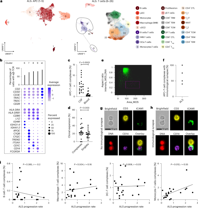
For imaging flow cytometry, cells were stained with the LIVE/DEAD Fixable Dead Cell Staining Kit (Life Technologies), blocked with an Fc receptor inhibitor and labeled with the following antibodies (fluorochrome, clone, provider, reference and amount used per 1 million cells): CD3+ (AF488, HIT3a, BioLegend, 300308, 5 μl), CD14 (BV421, HCD14, BioLegend, 325616, 1 μl), CD16 (BV786, 3G8, BD Biosciences, 557758, 5 μl), CD1c (BV711, REA694, Miltenyi Biotec, 130-110-537, 2 μl) and ICAM1 (FITC, REA266, Miltenyi Biotec, 130-129-412, 2 μl). Cells were fixed, permeabilized (eBioscience FoxP3/Transcription Kit, Invitrogen) and analyzed using ImageStreamX MkII (Amnis) at 40× magnification. IDEAS v6.2.183.0 software was used for analysis, and complexes were counted manually.
Statistical analysis
To evaluate whether T cell subsets were associated with longitudinal disease progression, linear mixed-effects models with random intercepts and random slopes were fitted using all available samples from 159 patients with ALS. ALSFRS-R score was modeled as the outcome, with time since sampling (expressed in 3-month intervals), T cell subset levels and their interaction included as fixed effects. Associations with ALSFRS-R decline were assessed using the estimated biomarker–time interaction coefficients, corresponding standard errors and P values. Analyses were adjusted for sex, age at sampling, site of onset, weight change from diagnosis to sampling and time from diagnosis to sampling.
The 6-month mortality following sampling was analyzed using logistic regression. To account for repeated measurements and varying numbers of observations per patient, within-cluster resampling was used42. In each iteration, one observation per patient was randomly selected and logistic regression models were fitted adjusting for sex, age at sampling, site of onset, weight change from diagnosis to sampling and disease progression rate at sampling. Disease progression rate was calculated as (48 − ALSFRS-R score) divided by the time from symptom onset to ALSFRS-R assessment (months). The resampling procedure was repeated 500 times, and regression coefficients were averaged across iterations.
The remaining statistical analyses were performed using GraphPad Prism version 10.6.1. All tests were two-tailed, and P < 0.05 was considered statistically significant. Comparisons between two independent groups were performed using the Mann–Whitney U test, while comparisons involving more than two groups were performed using the Kruskal–Wallis test. Associations between continuous variables were assessed using simple linear regression.
CMV antibody immunoblotting
For the viral antibody quantification, we used the recomLine CMV IgG [Avidität] (Mikrogen Diagnostik) kit according to manufacturer’s instructions. The kit determines antibody levels against six CMV antigens: IE1, CM2, p150, p65, gB1 and gB2. Serum samples of 706 patients with ALS were analyzed. The samples were collected between 1993 and 2020 and had been in long-term storage at −80 °C. The IE1 protein antibody data, marker of recent CMV activation, was included in this study. A separate larger article on viral antibodies in ALS will be prepared (project ongoing).
The Shapiro–Wilk test was used to check whether the data were normally distributed. We performed the analyses with the antibody levels both as semiquantitative (ternary analysis, 0, + and ++/+++) and as qualitative (negative versus positive) variables owing to the similarities in the antibody distributions. The ALS cohort was split into three categories according to genetic background: C9Exp group, genetically unknown group and SOD1*D91A homozygous group. Linear regression models were used to investigate the association between ALS survival and antibody levels. The models were adjusted according to the age of onset, gender and site of onset.
Reporting summary
Further information on research design is available in the Nature Portfolio Reporting Summary linked to this article.