Clinical usability of an explainable AI decision support tool and evaluation of multimodal models in NSCLC

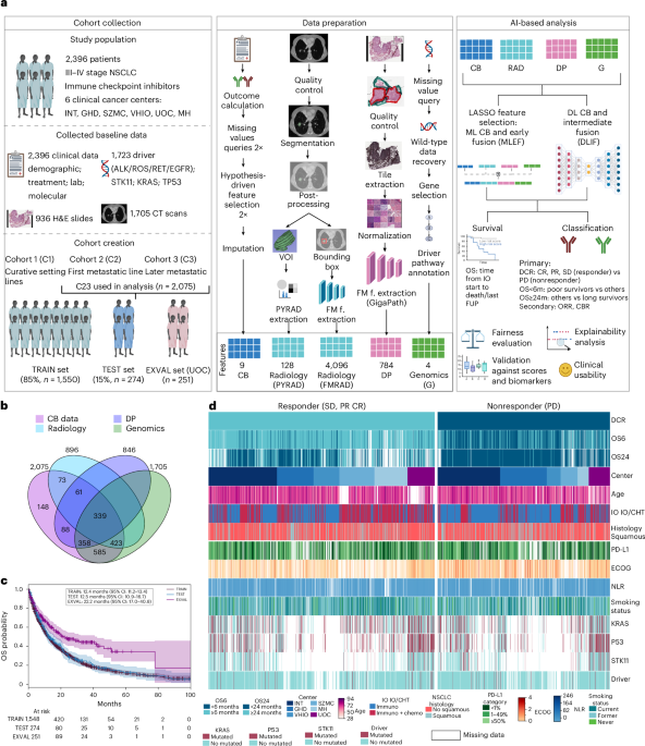
The I³LUNG project (NCT05537922) uses a two-phase approach to develop a medical device to predict IO efficacy in patients with NSCLC. This framework integrates multimodal clinical and multiomics data. Here we report the results from the retrospective phase, focused on developing a preliminary predictive model for IO outcomes that served as the foundation for the initial PDSS version.

Patient enrollment

This study included retrospective data from 2,396 patients with stage IIIC–IVB NSCLC who received IO-based therapy between September 2012 and October 2023 across 6 international institutions: INT-Italy, GHD-Germany, MH-Greece, SZMC-Israel, VHIO-Spain and UOC-USA. Patients with available baseline data and known clinical outcomes (response to IO according to Response Evaluation Criteria In Solid Tumors (RECIST) OS) were included in the analysis. All patients were enrolled as part of the I³LUNG international, multicenter, retrospective and prospective observational study (NCT05537922). Eligibility criteria included adults aged 18 years or older and a histologically confirmed diagnosis of stage IIIC–IVB NSCLC according to the 8th edition of the TNM staging system. The study was conducted in compliance with the Declaration of Helsinki and Good Clinical Practice guidelines, with ethics approval obtained at each participating site.

Clinical data

The study population was subdivided into three patient cohorts based on NSCLC disease stage:

• C1, Curative Setting: patients with stage III NSCLC treated with curative-intent chemoradiation therapy (concomitant or sequential) followed by maintenance IO.

• C2, Non-Curative Setting, First Metastatic Line: includes patients with advanced or metastatic NSCLC who received first-line IO, either alone or in combination with CHT or other therapeutic agents.

• C3, Non-Curative Setting, Later Lines: includes patients with advanced or metastatic NSCLC treated with IO in any line beyond first-line, either alone or in combination with CHT or other agents.

For patients who received IO in both curative and non-curative settings, their data were duplicated and included in both C1 and either C2 or C3, depending on their metastatic treatment line. CONSORT flow is shown in Extended Data Fig. 1a.

The data curation process began with involved hypothesis-driven feature selection, from more than 11,000 features from the electronic case report forms within the centralized I³LUNG platform. Features were categorized as (1) baseline features: CB and genomics features available before the administration of the first IO cycle and (2) treatment-related features: associated with treatment efficacy and toxicity. To reduce dimensionality, two independent blinded groups of oncologists (L.P. and C. Silvestri versus A.S. and C.G.) performed feature review and selection. A total of 227 features, including age at IO start and patient’s comorbidities (full list provided in Supplementary Information 1, Table 1), were consistently selected by both groups. These baseline IO features were further divided into (1) descriptive features, used for exploratory analysis and submodel development, and (2) predictive features, used to train the models. The final feature selection was performed by M.C.G. and A.P., senior oncologists with extensive experience in lung cancer treatment, resulting in a final set of nine CB features used for model development.

The second step focused on data cleaning and quality control, including standardization of free-text entries and correction of inconsistencies in dates and numerical values. Quality control was performed through three iterative validation rounds with participating centers to resolve missing values, inaccurate entries and dataset discrepancies, thereby improving overall data reliability and consistency.

New non-IO cohorts

To address the question of the predictive value of our models, we have collected and curated data from four additional cohorts; three of them are not part of the I³LUNG study. In detail:

1. 1.

   C-EGFR-INT: patients with EGFR-mutant NSCLC treated with EGFR-TKIs (from INT)

2. 2.

   C-EGFR-UOC: patients with EGFR-mutant NSCLC treated with EGFR-TKIs (from UOC)

3. 3.

   C-StageIII-CHT: patients with stage III NSCLC treated with neoadjuvant CHT (from INT) and followed by surgery

4. 4.

   C-LineI-CHT: patients from I³LUNG C3 who received first-line CHT before second-line IO (baseline CHT features used)

Clinical endpoints

We used two types of clinical endpoints to evaluate treatment efficacy: response outcomes and survival outcomes. Response outcomes were assessed using RECIST version 1.1, leading to the definition of the key response metric, DCR, where patients were classified as:

1. a.

   Nonresponders (class 0): progressive disease (PD)

2. b.

   Responders (class 1): stable disease (SD), partial response (PR) and complete response (CR)

We have used two additional response metrics:

1. 1.

   ORR:

   1. a.

      Nonresponders (class 0): PD and SD

   2. b.

      Responders (class 1): PR and CR

2. 2.

   CBR:

   1. a.

      Nonresponders (class 0): PD and SD with PFS < 6 months

   2. b.

      Responders (class 1): PR, CR and SD with PFS ≥ 6 months

We selected OS as the time from initiation of IO to death or last follow-up to assess treatment durability. Progression-free survival (PFS) was defined as the time from the initiation of IO therapy to disease progression or death.

The primary endpoints of the study included the identification of long responders (OS at 24 months (OS24)), poor responders (OS at 6 months (OS6)) and DCR for classification tasks and OS for survival analysis.

For both OS6 and OS24, we defined binary survival endpoints using a landmark approach:

1. 1.

   OS6:

   1. a.

      Class 0: patients who died within 6 months from treatment initiation

   2. b.

      Class 1: patients who survived ≥6 months

2. 2.

   OS24:

   1. a.

      Class 0: patients who died within 24 months

   2. b.

      Class 1: patients who survived ≥24 months

To avoid misclassification and follow-up bias, patients with follow-up shorter than the respective landmark time who were still alive at last contact were excluded from the corresponding analysis. This ensured that survival status at the landmark timepoint could be determined with certainty for all included patients.

The secondary endpoints of the study included ORR and CBR for classification tasks. Results on these endpoints are shown in Supplementary Information 2 (Figs. 1 and 2) and Supplementary Information 4 (Figs. 1 and 2).

Full statistical analysis of the CB across centers and cohorts is shown in Supplementary Information 1.

CT scans

CT scans were collected in Digital Imaging and Communications in Medicine (DICOM) format and underwent quality control, harmonization and segmentation. Scans were predominantly acquired at baseline prior to IO initiation. Given the real-world design of the study, when a baseline IO CT was unavailable or when the primary lesion was not present for a previous surgery, scans obtained at diagnosis were included.

Given the multicenter real-world design, CT acquisition was heterogeneous, and CT scans with missing metadata, usage of nonstandard or soft tissue kernels, artifacts, slice thickness out of the range 1–5 mm (for example, 10 mm), clinical exclusion (for example, patients with concurrent malignancies or without pulmonary lesion) and corrupted DICOM were excluded (Extended Data Fig. 1bii). Segmentations were performed in a three-dimensional slicer, using a semiautomated approach with manual refinement by a single trained radiologist. Difficult cases were reviewed by a senior radiologist (B.R.N.), ensuring consistent segmentation across all cases with no interoperator variability. The final segmentation masks were exported as NRRD files by the team at SZMC.

Of 896 CT scans used, 110 patients (12–33% in C2 and 77% in C3) did not have available pre-IO CT scan, and 41 (5–26% in C2 and 15% in C3) received surgery. For 23 patients (3–16% in C2 and 7% in C3), CT scans were collected after IO initiation. The distribution of time intervals between CT acquisition and IO initiation is provided in Supplementary Information 7, Fig. 1a. To assess their impact, we reran the models with and without these CT scans; performance remained stable, and multimodal improvements were maintained.

When available, contrast‑enhanced scans were preferred; of 896 CT scans, 758 (84.6%) were contrast, and 138 (15.4%) were noncontrast. Robustness analyses were performed to assess PYRAD features extracted from contrast versus noncontrast CT scans. Differences were observed, likely due to the limited number of noncontrast images (Supplementary Information 7, Robustness Analysis). However, excluding noncontrast images did not impact performance in either unimodal or selected multimodal models using PYRAD features. Available metadata analysis, with focus on manufacturer, slice thickness and contrast information of the included CT scans, is shown in Supplementary Information 7, Fig. 1bi–iii across TRAIN, TEST and EXVALl and in Fig. 1ci–iiiby center. To assess the robustness and discriminative power of radiomic features, we applied a contour randomization approach to each lesion segmentation delineated by the radiologist team at SZMC. For each lesion, we generated 10 randomized versions of the original mask, resulting in 11 segmentations per lesion (1 original + 10 perturbed). Radiomic features were extracted from each of these segmentations using PYRAD, resulting in 1,400 features per setting. To evaluate feature stability and relevance, we applied a statistical framework based on the inverse coefficient of selection, IS_f. This metric captures both intrasample robustness \({\sigma }_{\mathrm{intra},f}^{2}\) and intersample discriminability \({\sigma }_{\mathrm{inter},f}^{2}\). Let \(l\in \{1,\ldots ,L\}\), \(p\in \{1,\ldots ,P\}\), \(f\in \{1,\ldots ,F\}\) denote lesion, perturbation and feature indices, respectively. Formally, the inverse coefficient of selection, IS_f, is defined as follows:

where

and X_l,p,f is the value of the feature f for lesion l and perturbation p. σ_intra variance was computed by assessing the average variability of each feature across all perturbation settings for a given lesion, where lower intravariance indicates higher robustness. σ_inter variance was computed as the variance of each feature across all patients in the original setting, serving as a measure of discriminative power, where higher indicates better. Finally, IS_f is defined as the ratio of intravariance and intervariance, where lower values indicate more stable and discriminative features. Features were ranked by IS_f, and we then applied an iterative selection strategy to avoid redundancy: at each step, the next-best-ranked feature was added only if it was not highly correlated with any of the already selected features. This process ensured the selection of a compact, nonredundant set of 128 robust and informative radiomic features²⁵. Example of expert CT segmentation with perturbations is shown in Supplementary Information 7, Fig. 1d.

Regarding the FMRAD approach, we used a domain-specific foundation model developed for cancer imaging biomarker discovery²⁶ to extract high-level imaging features from CT scans. This model was pretrained using contrastive learning on a large dataset of 11,467 radiographic lesions, enabling it to learn generalized and transferable representations of tumor morphology. For our study, we applied this foundation model to volumetric image patches of size 50 × 50 × 50 mm, extracted around the centroid of the segmented primary lesion. The lesion center was determined from the segmentation mask, and the surrounding cubic volume was resampled and standardized as required by the foundation model input specifications. The resulting embeddings served as compact and expressive imaging descriptors for subsequent multimodal integration and predictive modeling. Future steps within the I³LUNG project include the development and evaluation of multi-lesion segmentation approaches to better capture disease heterogeneity and improve predictive performance.

DP

DP H&E slides were obtained at the time of diagnosis or at IO initiation; when biopsy material at IO start was available, it was preferentially used. The distribution of time intervals between biopsy and DP acquisition is shown in Supplementary Information 7, Fig. 2ai,ii. We compiled a total of 998 histopathological slides for our study, sourced from five institutions: 117 slides from GHD, 364 from INT, 81 from MH, 147 from SZMC and 191 from UOC. Of these, 64 slides were excluded from further analysis due to quality control concerns, such as insufficient tissue, physical damage (that is, scratched slides), poor staining quality and other technical artifacts that could compromise downstream analysis (CONSORT flow in Extended Data Fig. 1biii). Each remaining slide was individually reviewed, with systematic annotation of pen markings, scanner-induced artifacts and out-of-focus regions. For tumor region identification, we trained a segmentation model using The Cancer Genome Atlas (TCGA) dataset. Tile extraction was performed at ×20 magnification, followed by Reinhard normalization, targeting only areas within the segmented tumor regions while avoiding the previously annotated artifacts. We used Prov-GigaPath²⁷, a slide-based pretrained foundation model: first, to encode each extracted tile into a vector; then, to aggregate each bag of vectors into a single embedding representative of the whole slide Image. To determine whether our results were driven by our choice in DP feature extractor, we re-extracted 768-dimensional features using TITAN²⁸, a multimodal whole-slide foundation model pretrained using self-supervised learning on whole-slide images and vision-language alignment with pathology reports. We compared our results using GigaPath DP features to those extracted by TITAN across all three outcomes and modality combinations. Results were consistent with our primary analysis: substituting TITAN features did not yield significant improvement over the CB-only model in any outcome.

Genomics data

To include genomics data into our models, we first identified a core set of primary driver genes relevant to NSCLC: KRAS, TP53, STK11, ALK, EGFR, RET and ROS1 (ref.²⁹). Pathogenic alterations were annotated using three widely recognized databases: ClinVar³⁰ (via Varsome), Cancer Hotspot³¹ and OncoKB³². Given minor inconsistencies among databases, an alteration was classified as pathogenic only if at least two of the three sources agreed. For model construction, we encoded individual binary features for KRAS, TP53 and STK11, where 1 indicated a detected mutation, 0 indicated a wild-type allele and NA indicated missing testing information. Additionally, we created a composite ‘driver’ feature to capture actionable alterations relevant at the first line for a target therapy and associated with uncertain or limited evidence of benefit from IO and generally negative outcome (EGFR, ALK, ROS1 and RET). These features were coded as 1 if any of these were altered upon testing, 0 if at least one was tested and not altered and NA if no testing data were available. This approach helped reduce missingness, given the common practice of testing these genes together in clinical workflows, and aimed to preserve signal strength for modeling of IO response and survival.

Development of the AI tools

We evaluated two main AI approaches for treatment outcome prediction: MLEF and DLIF. The data preprocessing and analysis pipelines were identical for both methods.

As part of the CB used for model training, we included a curated set of clinical and biological features selected by two expert lung oncologists (M.G. and A.P.) for the main analysis reported in this paper. These included patient characteristics (sex, ECOG PS and smoking status), molecular features (PD-L1 expression), metastatic sites (bone, liver and brain) and laboratory values (NLR and LDH). Details on feature encoding are provided in Supplementary Information 1, Table 2. In addition, we have run the data-driven approach by selecting CB using least absolute shrinkage and selection operator (LASSO) starting from 227 features, because there was no significant difference in results (Supplementary Information 7, Table 1); here we report results obtained by using nine selected features as a starting point. Missing values were handled using multivariate imputation via the IterativeImputer (1.6.1). We used CV with each fold corresponding to a different center (that is, leave-one-center-out (LOCO)), resulting in a total of five CV folds.

We performed the main analysis on the combined C2 and C3 to increase the cohort size. Additionally, we performed several subgroup analyses to evaluate performance across clinically homogeneous subpopulations. These included models trained on C2, IO-only, IO/CHT, PD-L1 ≥ 50%, PD-L1 < 50%, PD-L1 1–49%, PD-L1 < 1%, P53, KRAS, STK11, squamous histology, adenocarcinoma histology and site-specific cohorts; summary of all analyses is in Supplementary Information 2, Table 1. For benchmarking, we compared model performance against individual clinical biomarkers, including PD-L1 expression, NLR, LDH and ECOG PS.

ML CB-only and MLEF

Before training the models, we performed feature selection using LASSO regression for FMRAD due to its high embedding dimensionality (more than 4,000 in length). For all other modalities, we started from the initial number of features (as shown in Fig. 1a); we concatenated them across all modalities; and we applied LASSO to select the most relevant predictors.

We implemented and evaluated two ML classifiers: (1) logistic regression and (2) random forest. We selected the optimal hyperparameters by maximizing the AUC during model tuning via Bayesian optimization. The best MLEF classifier was selected using CV AUC. All models were trained exclusively on the training cohort, using LOCO, and then applied directly to TEST and to the EXVAL cohort without threshold adjustment: a fixed decision threshold of 0.5 was used. In addition, to assess potential positive selection bias in the multimodal population, we conducted dedicated sensitivity analyses, which did not demonstrate evidence of systematic selection bias (Supplementary Information 2, Tables 2 and 3).

All performance results include 95% CI, and comparisons across models were conducted using DeLong’s test for AUC differences, with P values calculated using a two-sided z-test: NS (not significant), *P ≤ 0.05, **P ≤ 0.01, ***P ≤ 0.001, ****P ≤ 0.0001. To evaluate model performance against single biomarkers, we focused on a subset of TEST for which biomarker measurements were available.

For the survival analysis, we implemented a Cox proportional hazards model as baseline, using the ‘lifelines’ package in Python³³. Additionally, we evaluated two ML-based survival models (random survival forest (RSF) and gradient boosting survival (GBS)) implemented with scikit-survival³⁴. Because no differences between models were noted, all the results for survival analysis refer to the Cox model.

All performance results include 95% CI, and C-index differences were tested using bootstrapping (n = 1,000) with two-sided P values derived from the bootstrap distribution. Given the exploratory, retrospective nature of this study and the large number of subgroup analyses and pairwise comparisons performed, all such analyses are considered hypothesis generating. No adjustment for multiple comparisons was applied; all P values are nominal and should be interpreted in the context of multiple testing. Results from the independent TEST and EXVAL cohorts are considered the primary evidence of model generalizability.

Because the MLEF pipeline cannot handle patients with missing modalities, all multimodal models exclude these patients. For transparency, each MLEF multimodal model was reported along with the number of patients included in the analysis as well as the best model for that analysis, and it was compared to the unimodal CB-only matched model using the same patient subset.

DL CB-only and DLIF

Our second approach, DLIF, was designed to address the missing modalities across patient cohorts. We implemented a supervised intermediate fusion pipeline for both classification and survival prediction tasks, integrating CB, DP, RAD and genomics using an attention-based multiple instance learning (MIL) framework³⁵. In this framework, each patient is represented as a bag of vectors, allowing a variable number of instances per patient. This design is particularly well suited to complex oncological datasets, such as the I³LUNG retrospective cohort (Fig. 1b–d), where full multimodal coverage was available only for a subset of patients. Modality-specific encoders projected each modality into a shared embedding space, and a crossmodal reconstruction loss was incorporated during training to promote consistent and interpretable latent representations across modalities. Both loss functions combine a primary task-specific loss with a reconstruction loss component:

where λ is the reconstruction weight parameter. The reconstruction loss encourages the model to learn meaningful crossmodal representations by requiring it to reconstruct missing modalities from available ones. For a batch with N samples and M modalities, let \({x}_{m}^{(i)}\) be the input feature for sample i and modality m, \({\hat{x}}_{m,j}^{(i)}\) be the reconstruction of modality j from modality m for sample i and \({M}^{(i)}\in {\left\{0,1\right\}}^{M}\) be the modality mask indicating available modalities for sample i, and the reconstruction loss is computed as:

where the double summation ensures that only valid reconstructions (where both source and target modalities are available) contribute to the loss; the normalization by the count of valid reconstructions prevents bias when modalities are missing; and mean squared error (MSE) is computed as \(\mathrm{MSE}(\hat{x},x)=\frac{1}{d}{\sum }_{k=1}^{d}{({\hat{x}}_{k}-{x}_{k})}^{2}\) where d is the feature dimension. For multimodal classification tasks, the primary loss is cross-entropy:

where C is the number of classes; \({y}_{c}^{(i)}\) is the one-hot encoded ground truth for sample i and class c; and \(\sigma \left({z}^{\left(i\right)}\right)\) is the softmax of the model’s logits for sample i. Optional class weights \(w\in {R}^{C}\) can be applied:

For survival analysis, the primary loss uses the Cox proportional hazards model:

where h_i is the log-hazard prediction for sample i; δ_i is the event indicator (1 if event occurred, 0 if censored); and \({R}_{i}=\left\{j:{T}_{\!j}\ge {T}_{i}\right\}\) is the risk set (samples with survival time ≥T_i). Samples are sorted by descending survival time for computational efficiency. To prevent overflow in the exponential operations, the log-sum-exp trick is used:

where \(\gamma ={\max }_{j\in {R}_{i}}{h}_{\!j}.\)

This design constraint promotes information alignment across modalities and effective fusion through the MIL attention mechanism.

Fairness evaluation

To assess fairness, we conducted a post hoc auditing focusing on potential biases across subgroups in TEST and EXVAL. We used center and sex as protected attributes for TEST and race and sex for EXVAL.

To quantify fairness, for classification models, we used equalized odds, which requires that both TPR (also known as sensitivity) and FPR are consistent across subgroups. TPR and FPR were calculated for the best-performing CB-only MLEF model.

For survival analysis models, we applied parity in C-index to verify whether model discrimination remained consistent across centers.

Fairness was evaluated using statistical tests to compare model performance across subgroups. For the classification tasks, we performed a permutation test with 1,000 iterations; for the survival task, we used bootstrapping with n = 1,000. In both cases, P values were calculated using a two-sided test for comparison between the two groups.

Per-center calibration analysis was conducted on the ML CB-only (logistic regression C23) model, selected as the case showing the largest statistically significant difference in TPR (P < 0.05). For each center, intercept recalibration was performed by fitting a logistic regression on the LOCO held-out set of that center, adjusting only the intercept while keeping all other model parameters fixed; this choice preserves the discriminative structure learned on the full cohort while correcting for center-specific shifts in the predicted probability scale. The recalibrated model was then evaluated on the corresponding center’s test subset. Classification metrics (TPR, FPR, sensitivity and specificity) were computed before and after recalibration for each of the five centers (GHD, INT, MH, SZMC and VHIO), and results are reported in Supplementary 5, Section 1, Table 2.

Explainability

Explainability analysis was conducted using SHAP³⁶. For each clinical endpoint, selecting the best-performing model, we generated summary SHAP plots trained on the TRAIN and applied both on the TRAIN and TEST. In addition, we produced individual waterfall plots for each patient in the TEST. These graphs are included in either the main text (Fig. 4c) or Extended Data Fig. 5, and these types of graphs were also used for the clinical usability study.

In the global SHAP summary plots, each point represents one patient, and the position on the x axis reflects the direction and magnitude of that feature’s contribution to the model output (for example, on Fig. 4c(i), positive SHAP values indicate a contribution toward class 1 (OS ≥ 24 months), whereas negative SHAP values indicate a contribution toward class 0 (OS < 24 months)). Features are ordered by mean absolute SHAP value, representing their overall importance across the cohort. In the individual waterfall plots (local explanations; Fig. 4c(iii)–(vi)), SHAP values illustrate how each feature shifts the prediction from the baseline (average model output) to the final predicted probability for a specific patient, thereby highlighting the key drivers of that individual prediction.

To identify the most influential features across outcomes, we created a summary graph (Fig. 4c(ii)) by calculating mean-ranked feature importance based on SHAP global values across all outcomes—the higher the rank, the higher the feature importance across analysis.

Clinical usability with ML CB-only model

The primary objective of the clinical usability study was to assess the clinical applicability of the I³LUNG tool. The clinical usability patient cohort consisted of 100 patients, of whom 35 had CT scans available, and 42 had H&E slides available. Patients were stratified into subgroups randomly.

The study involved 20 medical oncologists, consisting of 10 expert lung oncologists and 10 nonexperts in lung cancer (including resident doctors and general oncologists) from the five centers (INT, VHIO, GHD, MH and UOC) from the consortium. Each patient was evaluated by one lung expert and one nonexpert, with each physician evaluating a total of 10 patients.

The study design consisted of two evaluation phases (Fig. 5). In phase 1, medical oncologists had access to important clinical data (all nine CB features plus other medical relevant characteristics; Supplementary Information 1, Table 1), segmented CT scan slice (when available) and DP slide. In phase 2, they had access to the available data and models output with global and local SHAP explanations. Supporting material provided to medical oncologists who were participating in the study is available in Supplementary Videos 1 and 2, including the tutorials on how to read the model’s explanation (tutorials for global and local explainability with SHAP). Patient evaluations were conducted based on two key outcomes: prediction of treatment response (DCR) and of survival (OS).

For treatment response, physicians categorized each patient as either a responder (CR, PR or SD) or a nonresponder (PD), following DCR RECIST³⁷. For survival, physicians assigned each patient to one of five predefined OS time intervals: <6, 6–12, 12–18, 18–24 and ≥24 months, and the tool generated an individual OS probability curve for each patient.

To evaluate the impact of XAI and physician expertise on prediction performance, we performed a series of univariable logistic regression analyses. For DCR, two models were run, and, in both cases, the outcome was binary, indicating prediction success (1: correct prediction; 0: incorrect). In the first analysis, to assess the effect of XAI, we used phase as the covariate (0: no XAI, phase 1; 1: with XAI, phase 2); for the second analysis, to assess the effect of physician expertise, we used expertise level as the covariate (0: non-lung-expert oncologist; 1: lung expert oncologist). For OS prediction, success was defined as whether the predicted OS range overlapped with the true OS ± 25% interval (1: overlap; 0: no overlap). The ±25% margin was selected to apply a stricter and more conservative definition of prediction accuracy, ensuring consistency between model outputs and clinicians’ broad survival categories while avoiding artificial inflation of predictive performance. Similarly, two univariable logistic regression models were applied: first, to test the effect of XAI use, where phase was used as the covariate; second, to assess the role of expertise, the covariate was (0: non-lung-expert oncologist; 1: lung expert oncologist). All models were run for the full physician group and separately for experts and nonexperts. All the results are presented as odds ratio and AUC with their 95% CI and are shown in Supplementary Information 6.

The degree of agreement between the expert and nonexpert physicians’ DCR and OS evaluations was assessed by computing the Cohen’s κ and the weighted Cohen’s κ, respectively. Based on the observed κ, the degree of concordance was considered as follows:

– 0: no agreement

– (0.01–0.20): slight agreement

– (0.21–0.40): fair agreement

– (0.41–0.60): moderate agreement

– (0.61–0.80): substantial agreement

– (0.81–0.99): near-perfect agreement

– 1: perfect agreement

McNemar’s test for paired data was employed to assess any differences between experts and nonexperts in the discordant predictions in phase 1 and phase 2.

Furthermore, sensitivity, specificity, accuracy, precision and F1 were computed for the DCR prediction according to phase and physicians’ expertise. The 95% CIs of these metrics were calculated by using the Clopper–Pearson exact binomial method. McNemar’s test for paired data was employed to assess any statistically significant differences. The F1 score was derived according to phase and physicians’ expertise for the DCR prediction. Its 95% CI was computed by using bootstrap methods with 1,000 replications.

Due to the time-to-event nature of the OS, conventional classification metrics based on true positives and true negatives could not be applied. Therefore, we defined a patient-level correctness score based on the agreement between the true OS and the physician’s predicted OS ranges as follows:

– 0 points were assigned in case of different and nonconsecutive ranges for the true OS and the predicted OS by the physician.

– 1 point was assigned in case of different, but consecutive, ranges for the true OS and the predicted OS by the physician.

– 2 points were assigned in case of identical ranges for the true OS and the predicted OS by the physician.

The Wilcoxon signed-rank test for paired data was employed to assess any statistically significant differences between the assigned scores’ distributions. A total correctness score was computed by summing all scores according to phase and physicians’ expertise.

Finally, the confusion matrix after using XAI³⁸ was derived for all physicians, for experts only and for nonexperts only (Fig. 5c and Supplementary Information 6, Tables 38–40). When a medical oncologist decides with the assistance of the XAI tool, four errors can occur: (1) false confirmation error (FCoE), (2) false conflict error (FCE), (3) true conflict error (TCE) and (4) true confirmation error (TCoE). Furthermore, in case of correct prediction, there are four possible scenarios: (1) correct true confirmation case (CTCo), (2) correct true conflict case (CTC), (3) correct false confirmation case (CFCo) and (4) correct false conflict case (CFC). All are summarized and explained in Supplementary Information 6, Table 1.

Ethics committee details

IO cohorts obtained approval from all of the centers within the I³LUNG study protocol:

1. 1.

   Comitato etico Fondazione IRCSS Istituto Nazionale dei Tumori (INT), ethics committee code 147/22, approved on 25 July 2022

2. 2.

   Ethik-Kommission Universitäumalt zu Lübeck (GHD), ethics committee code 2022-439, approved on 17 October 2022 (clinical study)

3. 3.

   Scientific Committee Metropolitan Hospital (MH), ethics committee code 30.08.2022, approved on 30 August 2022

4. 4.

   Helsinki Committee Share Zedek Medical Center (SZMC), ethics committee code 0240-22-SZMC, approved on 20 September 2022

5. 5.

   Comité de Ética de Investigación con medicamentos y Comisión de Proyectos de Investigación del Hospital Universitari Vall D’Hebron, approved on 17 January 2023

6. 6.

   Institutional Review Board University of Chicago (UOC), ethics committee code IRB22-1305, approved on 8 September 2022

Non-IO cohorts

C-EGFR-INT: These data were collected within the APOLLO 11 study and approved by the ethics committee of INT (reference no. INT 128/22) on 29 June 2022.

C-EGFR-UOC: Institutional Review Board University of Chicago (UOC), ethics committee code IRB24-2188, approved on 23 December 2024

C-StageIII-CHT: For this cohort collected in INT, the data protection impact assessment was developed and is published at the INT website https://dpm.istitutotumori.mi.it/public/documents/ (called Informativa-I³LUNG Monocentrico), in compliance with applicable personal data protection laws, including Regulation (EU) 2016/679 (General Data Protection Regulation) and relevant national legislation. A distinct and appropriate legal basis was identified for each category of personal data processed, tailored to the nature and purpose of each specific processing activity. Suitable technical and organizational measures were put in place to ensure an adequate level of data security, in line with the principles of data minimization, purpose limitation and access control, ensuring that only authorized individuals were granted access to personal information. The research was carried out in accordance with applicable ethical standards and under the supervision of the relevant institutional bodies. Throughout the entire research process, the accountability principle was upheld, meaning that the data controller was not only committed to complying with data protection requirements but was also in a position to demonstrate such compliance at any time.

Generative AI tools, specifically GPT-5.3, were used for English language editing to improve the clarity of this paper. The AI-assisted language editing was performed under human oversight, and the final paper was thoroughly reviewed and edited by the authors to ensure accuracy and integrity. All intellectual content, literature analysis and scientific conclusions were conducted by the authors.

Reporting summary

Further information on research design is available in the Nature Portfolio Reporting Summary linked to this article.