Sex-specific biological aging clocks across organs and omics

Method 1: The MULTI study

The MULTI Consortium is an ongoing initiative to integrate and consolidate multi-organ and multi-omics data, including imaging, genetics and proteomics. Building upon existing consortia and studies, MULTI aims to curate and harmonize the data to model human aging and disease at scale across the lifespan. See Supplementary Table 1 for comprehensive information, including the complete list of data analyzed and their respective sample characteristics. Participants provided written informed consent to the corresponding studies. The MULTI study is approved by the institutional review board at Columbia University (AAAV6751).

UKBB

The UKBB⁴⁴ is a population-based research initiative comprising approximately 500,000 individuals from the United Kingdom between 2006 and 2010. Ethical approval for the UKBB study has been secured, and information about the ethics committee can be found here: https://www.ukbiobank.ac.uk/learn-more-about-uk-biobank/governance/ethics-advisory-committee. This study retrained biological aging clocks in a sex-stratified manner. The seven brain MRIBAGs⁸ were derived from multi-organ MRI data at the second visit; 11 ProtBAGs⁷ and five MetBAGs¹⁴ were derived using plasma proteomics and metabolomics at baseline. We also incorporated inpatient disease diagnoses and mortality records into the survival analyses.

Baltimore Longitudinal Study of Aging

The main goal of the Baltimore Longitudinal Study of Aging (BLSA) is to understand the normal aging process. Tracking physiological and cognitive changes over time aims to identify risk factors for age-related diseases, study patterns of decline and discover predictors of healthy aging. BLSA^45,46 brain MRI and SomaScan proteomics data (https://www.blsa.nih.gov/) were used to compare and replicate the ProWAS results from the UKBB Olink data. After quality checks in this study, we included 1,114 brain MRI scans at baseline and measurements of 7,268 plasma proteins from 909 participants quantified with the SomaScan version 4.1 platform. Age (years), sex (male/female), race (white/non-white) and education level (years) were defined based on participant self-reports.

A4

The A4 study²⁴ (https://atri.usc.edu/study/a4-study/) is a clinical trial study to test a specific way to prevent memory loss associated with AD (clinical trial number: NCT02008357). The A4 study focused on symptom-free adults at higher risk for AD to assess whether an investigational drug (that is, solanezumab) could slow memory decline linked to amyloid plaques in the brain. It also examined whether solanezumab could delay AD progression, measuring related brain changes using imaging, blood biomarkers and baseline positron emission tomography (PET) scans to assess amyloid levels. This study analyzed 1,055 participants at baseline with brain MRI scans to derive the brain MRIBAG. Longitudinal outcomes from the clinical trial, with the PACC score as the primary measure over 312 weeks, were included. The PACC scores between groups were evaluated at week 240. We used the A4 trial data to test for sex differences between female and male participants, stratifying them into accelerated (brain MRIBAG > 0) and decelerated (brain MRIBAG ≤ 0) brain agers, as we previously showed heterogeneity in the drug outcome⁸.

ADNI

The ADNI²³ (https://adni.loni.usc.edu/) includes patients from different stages of the disease progression: CN individuals, those with MCI and those with AD. This allows researchers to compare brain structure and function changes across the AD continuum. We included baseline brain MRI data of 1,765 individuals and 9,752 longitudinal follow-up scans (at least >5 brain MRI scans for the same participant). The ADNI longitudinal data were used for the CN → MCI and MCI → AD progression analyses.

FinnGen

The FinnGen⁴⁷ study is a large-scale genomics initiative that has analyzed more than 500,000 Finnish biobank samples and correlated genetic variation with health data to understand disease mechanisms and predispositions. The project is a collaboration between research organizations and biobanks within Finland and international industry partners. For the benefit of research, FinnGen generously made its GWAS findings accessible to the wider scientific community (https://www.finngen.fi/en/access_results). This research utilized the publicly released GWAS summary statistics (version R9), which became available on 11 May 2022, after harmonization by the consortium. No individual data were used in the present study.

FinnGen published the R9 version of GWAS summary statistics via REGENIE software (version 2.2.4)⁴⁸, covering 2,272 DEs, including 2,269 binary traits and three quantitative traits. The GWAS model encompassed covariates such as age, sex, the initial 10 genetic principal components and the genotyping batch. Genotype imputation was referenced on the population-specific SISu version 4.0 panel. We included GWAS summary statistics for 521 FinnGen DEs in our analyses.

PGC

The PGC⁴⁹ is an international collaboration of researchers studying the genetic basis of psychiatric disorders. The PGC aims to identify and understand the genetic factors contributing to various psychiatric disorders such as schizophrenia, bipolar disorder, major depressive disorder and others. The GWAS summary statistics were acquired from the PGC website (https://pgc.unc.edu/for-researchers/download-results/), underwent quality checks and were harmonized to ensure seamless integration into our analysis. No individual data were used from the PGC. Each study detailed its specific GWAS models and methodologies, and the consortium consolidated the release of GWAS summary statistics derived from individual studies. In the present study, we included summary data for six brain diseases.

Method 2: Machine learning models for the sex-specific biological aging clocks

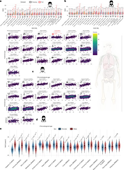
In our previous work, we derived a total of 23 BAGs^7,8,14. We also benchmarked age prediction using multiple machine learning approaches, including linear regression, support vector regression, neural networks and LASSO regression, and found no evidence that any single model consistently outperformed the others. In the present study, we used LASSO regression as a linear model and a neural network as a nonlinear model, training the model separately in females and males. Consistent with our previous work on brain age, we found that sex-stratified models tended to exhibit more pronounced overfitting¹⁵.

To rigorously benchmark model performance, all 46 BAGs (23 for each sex) were developed using a nested cross-validation framework, adhering to best practices in machine learning to minimize overfitting and prevent data leakage^7,50. We split the data into the following datasets:

• CN within-distribution, hold-out test dataset: For each sex, approximately 250 participants for MRIBAGs and ProtBAGs and 2,500 for MetBAGs were randomly drawn from the CN population. Within-distribution, hold-out test datasets are ideal for objectively evaluating AI model performance, especially in studies with large sample sizes such as the UKBB.

• CN training/validation dataset: Eighty percent of the remaining CN population was used for the inner loop 10-fold cross-validation for hyperparameter selection.

• CN cross-validation test dataset: Twenty percent of the remaining CN population was used for the outer loop for 50 repetitions.

• PT dataset: This includes all patients who have at least one International Classification of Diseases (ICD)-based diagnosis.

The age distribution for the CN CN training/validation datasets and CN within-distribution, hold-out test dataset for each organ aging clocks between females and males is presented in Supplementary Table 6.

Evaluation metrics for age prediction models

Within our cross-validation framework, we report three complementary metrics to characterize model performance: (1) MAE, (2) Pearsonʼs r and (3) R². MAE quantifies the average absolute prediction error in years and, therefore, reflects individual-level accuracy; Pearsonʼs r measures the linear association between predicted and chronological age and reflects how well the model preserves age ranking across individuals; and R² quantifies the proportion of age variance explained by the model relative to a mean age baseline, capturing overall predictive accuracy and calibration. These metrics are reported in the main paper using the original predicted ages before age bias correction, whereas all downstream association analyses were performed using BAGs after age bias correction.

Comparative analysis to compare sex-specific/stratified models and sex-pooled models

We performed direct comparative analyses using the same cross-validation framework and matched training sample sizes and age distributions. Specifically, we compared the two training strategies in the CN training/validation/test datasets: (1) female-only or male-only models and (2) sex-pooled models downsampled to match the sample size and age distribution of the corresponding female-only or male-only training set. For age prediction evaluation in the within-distribution, hold-out test dataset, we used eight different schemes: (1) female-trained models tested in females, (2) female-trained models tested in males, (3) male-trained models tested in males, (4) male-trained models tested in females, (5) sex-pooled (femalesʼ sample size matched) models tested separately in females, (6) sex-pooled (femalesʼ sample size matched) models tested separately in males, (7) sex-pooled (malesʼ sample size matched) models tested separately in females and (8) sex-pooled (males’ sample size matched) models tested separately in males.

Method 3: Genetic analyses

We used the genotype and imputed genotype data from the UKBB for all genetic analyses. Our quality check pipeline focused on European ancestry in the UKBB (6,477,810 SNPs passing quality checks). We summarize our genetic quality check steps. First, we excluded related individuals (up to second degree) from the complete UKBB sample using KING software for family relationship inference⁵¹. We then removed duplicated variants from all 22 autosomal chromosomes. Individuals whose genetically identified sex did not match their self-acknowledged sex were removed. Other exclusion criteria were as follows: (1) individuals with more than 3% of missing genotypes; (2) variants with minor allele frequency (MAF; dosage mode) of less than 1%; (3) variants with more than 3% missing genotyping rate; and (4) variants that failed the Hardy−Weinberg test at 1 × 10⁻¹⁰. To further adjust for population stratification⁵², we derived the first 40 genetic principal components using FlashPCA software⁵³. Details of the genetic quality check protocol are described elsewhere^{15,20,54,55,56}.

Sex-stratified GWAS

We applied a linear mixed model regression to the European ancestry populations using fastGWA⁵⁷ implemented in GCTA⁵⁸. Our GWASs adjusted common covariates, including age, dataset status (training/validation/test or within-distribution, hold-out test), age-squared, sex, interactions of age with sex, body mass index (BMI), waist circumference, standing height, weight and the first 40 genetic principal components as well as organ-specific covariates, including the brain scan positions for the brain MRIBAG and systolic/diastolic blood pressure for the heart MRIBAG. We applied a stringent threshold based on Bonferroni correction at the genome-wide significance level (5 × 10⁻⁸/15 organs) to annotate the significant independent genomic loci.

Annotation of genomic loci

For all GWASs, genomic loci were annotated using FUMA⁵⁹. For genomic loci annotation, FUMA initially identified lead SNPs (correlation r² ≤ 0.1, distance <250 kilobases) and assigned them to non-overlapping genomic loci. The lead SNP with the lowest P value (that is, the top lead SNP) represented the genomic locus. Additional details on the definitions of top lead SNP, lead SNP, independent significant SNP and candidate SNP can be found in Supplementary Note 1.

Three key genetic parameters

We used SBayesS⁶⁰ to estimate three key genetic parameters that characterize the genetic architecture of the 38 BAGs. SBayesS is an expanded approach capable of estimating three essential parameters characterizing the genetic architecture of complex traits through a Bayesian mixed linear model⁶¹. This method only requires GWAS summary statistics of the SNPs and linkage disequilibrium information from a reference sample. These parameters include SNP-based heritability (h²), polygenicity (Pi) and the relationship between MAF and effect size (S) as natural selection signatures. We used the software pre-computed sparse linkage disequilibrium correlation matrix derived from the European ancestry by Zeng et al.⁶⁰. More mathematical details can be found in the original paper from Zeng et al.⁶⁰.

SBayesS is a pure Bayesian method. To compare the estimated parameters within the same organ-specific BAG between males and females, we fitted SBayesS in GCTB to obtain the posterior mean and posterior standard deviation (s.d.) of the three parameters. Taking h² as an example, to quantify sex differences in \({h}^{2}\) for a given BAG, we defined \({\Delta }{h}^{2}={h}_{\text{female}}^{2}-{h}_{\text{male}}^{2}\). Assuming approximate normality and independence of the sex-specific posterior estimates, we computed the s.d. of this difference as \({\rm{s}}.{\rm{d}}.({\Delta }{h}^{2})=\sqrt{{\rm{s}}.{\rm{d}}.{({h}_{\text{female}}^{2})}^{2}+{\rm{s}}.{\rm{d}}.{({h}_{\text{male}}^{2})}^{2}}\). A 95% credible interval for \(\Delta {{\rm{h}}}^{2}\) was then given by \({\Delta }{h}^{2}\pm 1.96\times {\rm{s}}.{\rm{d}}.({\Delta }{h}^{2})\); sex differences were considered supported when this interval did not include zero (either >0 or <0).

Two-sample bidirectional Mendelian randomization

We constructed two-sample bidirectional Mendelian randomization by linking the 38 sex-specific BAGs and 525 DEs from FinnGen⁴⁷ and PGC⁴⁹ (two DEs from PGC did not provide allele frequency information). In total, two networks were established: (1) BAG2DE and (2) DE2BAG. We performed systematic quality-checking procedures to ensure unbiased exposure/outcome variable and instrumental variable selection.

We used the TwoSampleMR package⁶² to infer the causal relationships within these networks. We employed five distinct Mendelian randomization methods, including the inverse variance weighted (IVW) method, Egger, weighted median, simple mode and weighted mode estimators. The STROBE-MR statement⁶³ guided our analyses to increase transparency and reproducibility, encompassing the selection of exposure and outcome variables, reporting statistics and implementing sensitivity checks to identify potential violations of underlying assumptions. First, we performed an unbiased quality check on the GWAS summary statistics. Notably, the absence of population overlapping bias⁶⁴ was confirmed, given that FinnGen and UKBB participants largely represent populations of European ancestry without explicit overlap with the UKBB. PGC GWAS summary data were ensured to exclude UKBB participants. Furthermore, the GWAS summary statistics of all consortia were based on or lifted to GRCh37. Subsequently, we selected the effective exposure variables by assessing the statistical power of the exposure GWAS summary statistics in terms of instrumental variables, ensuring that the number of instrumental variables exceeded seven before harmonizing the data. Crucially, the function clump_data was applied to the exposure GWAS data, considering linkage disequilibrium. The function harmonise_data was then used to harmonize the GWAS summary statistics of the exposure and outcome variables. Bonferroni correction was applied across all tested traits based on the number of effective DEs and BAGs, resulting in a relatively conservative adjustment.

Finally, we conducted multiple sensitivity analyses. First, we conducted a heterogeneity test to scrutinize potential violations of the instrumental variableʼs assumptions. To assess horizontal pleiotropy, which indicates the instrumental variableʼs exclusivity assumption⁶⁵, we utilized a funnel plot, single-SNP Mendelian randomization methods and the Egger estimator. Furthermore, we performed a leave-one-out analysis, systematically excluding one instrument (SNP/instrumental variable) at a time, to gauge the sensitivity of the results to individual SNPs.

Genetic correlation

We estimated the genetic correlation (g_c) using LDSC²⁷ software (1) between each pair of BAGs and (2) between the BAG and 527 DEs from the FinnGen and PGC datasets. We employed pre-computed linkage disequilibrium scores from the 1000 Genomes of European ancestry, maintaining default settings for other parameters in LDSC. It is worth noting that LDSC corrects for sample overlap, ensuring an unbiased genetic correlation estimate⁶⁶.

Method 4: Sex-stratified proteome-wide associations

We used the original dataset (Category ID: 1838), which was analyzed and shared with the research community by the UK Biobank Pharma Proteomics Project (UKB-PPP)⁶⁷. The initial quality control procedures were described in the original study⁶⁸, and we implemented additional quality control steps as outlined below. Our analysis focused on the first instance of the proteomics data (‘instance’ = 0). We then integrated Olink files containing coding information, batch numbers, assay details and limit of detection (LOD) data (Category ID: 1839) by matching them to the proteomics dataset ID. Finally, we excluded normalized protein expression (NPX) values that fell below the protein-specific LOD. Descriptions of these proteins are provided in our previous study⁷.

We conducted ProWASs by linking the seven MRIBAGs to 2,923 unique plasma proteins in a linear regression model. The model was adjusted for common covariates, including age, sex, weight, height, waist circumference, BMI, assessment center, disease status, diastolic and systolic blood pressure, protein batch number, LOD and the first 40 genetic principal components. To identify and exclude extreme outliers, we defined an upper threshold as the mean plus four times the standard deviation for each protein.

We also conducted secondary analyses that included 13 female-specific variables: ever had breast cancer screening/mammogram (Field ID: 2674), ever had a cervical smear test (Field ID: 2694), age at menarche (Field ID: 2714), age at menopause/last menstrual period (Field ID: 3581), number of live births (Field ID: 2734), birth weight of first child (Field ID: 2744), age at first live birth (Field ID: 2754), age at last live birth (Field ID: 2764), history of stillbirth (Field ID: 3829), miscarriage (Field ID: 3839) or termination (Field ID: 2774), age at starting oral contraceptive use (Field ID: 2794), ever used hormone replacement therapy (Field ID: 2814) and history of hysterectomy (Field ID: 3591) and bilateral oophorectomy (Field ID: 2834). These variables were included to capture sex-specific reproductive and hormonal transitions that might confound or mediate associations with biological aging, thereby yielding more accurate and interpretable estimates in women. However, these measures are available for only 78,784 participants, substantially reducing statistical power. After merging with the BAG populations, we could perform these analyses only for the digestive, metabolic, immune and hepatic MetBAGs. To ensure a fair sex-stratified comparison with similar power (that is, similar sample sizes) between females and males, we, therefore, present these results as secondary analyses.

Method 5: Sex-stratified metabolome-wide associations

We used the original data (Category ID: 220), which were analyzed and made available to the community by Nightingale Health Plc. The original data (1) were calibrated absolute concentrations (or ratios) and not raw nuclear magnetic resonance (NMR) spectra and (2), before release, had already been subject to quality control procedures by Nightingale Health Plc⁶⁹. After the additional procedures described in Ritchie et al.⁷⁰, we performed additional quality check steps to remove a range of unwanted technical variations, including shipping batch, 96-well plate, well position, aliquoting robot and aliquot tip. We focused our analysis on the first instance of the metabolomics data (‘instance’ = 0). The analysis included 327 metabolites (comprising both small molecules and lipoprotein measures), of which 107 were non-derived metabolites and the remainder were composite metabolites, across 274,247 participants. Descriptions of these metabolites are provided in our previous study¹⁴.

We conducted MetWASs by linking sleep duration to the 107 non-derived plasma metabolites and/or lipoproteins. The linear regression model controlled common covariates, including age, sex, weight, height, waist circumference, BMI, assessment center, disease status, diastolic and systolic blood pressure and the first 40 genetic principal components. To identify and exclude extreme outliers, we defined an upper threshold as the mean plus four times the standard deviation for each metabolite.

Method 6: Sex-stratified survival analyses for future onset of DEs, all-cause mortality and AD progression

Using longitudinal data from inpatient medical records and baseline MRI scans, we conducted time-to-event prediction with survival analyses.

Survival analysis for ICD-based single DE

We employed a Cox proportional hazards model while adjusting for covariates (for example, age) to test the associations of the 38 sex-specific BAGs with the time to incident of ICD-based single disease entities. The covariates age, BMI, height, weight, waist circumference, smoking status and blood pressure were included as additional right-side variables in the model. To train the model, the ‘time’ variable was determined by calculating the difference between the date of diagnosis of the disease for cases (or the censoring date for non-cases) and the date of attendance at the assessment center. Participants who were diagnosed with a specific disease of interest after enrolling in the study were classified as cases; non-cases were defined as participants without any disease diagnoses.

Survival analysis for mortality risk

We employed a Cox proportional hazards model while adjusting for covariates (for example, age) to test the associations of the 38 sex-specific BAGs with all-cause mortality. The covariates age, BMI, height, weight, waist circumference, smoking status and blood pressure were included as additional right-side variables in the model. The hazard ratio, exp(β_R), was calculated and reported as the effect size measure that indicates the influence of each biomarker on the risk of mortality. To train the model, the ‘time’ variable was determined by calculating the difference between the date of death for cases (or the censoring date for non-cases) and the date attending the assessment center. Participants who died after enrolling in the study were classified as cases.

Survival analysis for AD disease progression

We used longitudinal data from the ADNI to evaluate whether sex-specific brain MRIBAGs predict clinical progression from CN to MCI and from MCI to AD. The brain age model was independently trained in ADNI to avoid potential domain shift. For CN → MCI, we first restricted to participants whose baseline diagnosis was CN and defined the CN baseline as the earliest CN visit per participant. We then followed each individual forward and identified the first visit at which the diagnosis changed to MCI. Time-to-event was defined as the difference in years between age at baseline CN and age at first MCI diagnosis; participants who did not convert were censored at their last observed age. For MCI → AD, we applied the same procedure starting from the first MCI visit as baseline and used the time from MCI baseline age to first AD diagnosis (or last follow-up for censored participants). Within each sex, we standardized the brain MRIBAG (z-score) and fitted Cox proportional hazards models with time in years as the time scale, MRIBAG as the main predictor (per 1-s.d. increase) and baseline age as an additional covariate, along with intracranial volume. Supplementary Kaplan−Meier curves were generated by stratifying either on sex within the CN or MCI group at baseline and comparing survival functions with log-rank tests.

Method 7: A4 drug analyses to test whether sex affects cognitive decline trajectories

We used data from the A4 trial to test whether brain MRIBAG modifies sex differences in treatment-related cognitive change on the PACC in the solanezumab trial data. The brain age model was independently trained in A4 to avoid potential domain shift. First, we restricted to participants randomized to solanezumab and extracted longitudinal PACC scores. For each participant, we used the sex-appropriate MRIBAG and classified individuals as accelerated (brain MRIBAG > 0) or decelerated (brain MRIBAG ≤ 0) brain agers. Within each brain-aging stratum, we modeled PACC trajectories using generalized least squares with a natural cubic spline for time since randomization, including a time-by-sex interaction and adjusting for baseline age, amyloid positivity, years of education, baseline amyloid PET (standardized uptake value ratio (SUVR)) and PACC version. From these models, we estimated (1) mean change in PACC from baseline to week 240 within each sex and (2) the female−male difference in PACC at week 240 and generated sex-specific predicted PACC trajectories with 95% confidence intervals separately for accelerated and decelerated brain agers.

Method 8: Logistic regression to link the sex-specific BAGs with medication status

We assessed the association between 38 sex-specific BAGs and medication use. Medication use for 163 drugs was determined by the UKBB Field ID (20003), and data were restricted to at least 50 cases. For each medication use case, the non-case group included individuals who had no recorded exposure to any available medications, and the case group included participants who only took the target medication.

To derive the incremental R² indicating the additional prediction power provided by the BAG, we built a null and an alternative logistic regression using the statsmodels package. The null model predicted medication status based on BMI, height, weight, waist circumference, smoking status, disease status and blood pressure as features, whereas the alternative model included each sex-specific BAG as an additional feature. The difference between the R² pseudo-values for the alternative and null models reflected the incremental R² explained by the BAG.

Reporting summary

Further information on research design is available in the Nature Portfolio Reporting Summary linked to this article.